Screen shot #3 (Merely a picture to illustrate that our GUI is totally self-explanatory)

Select the data source and processing architecture from the indicated menu appearing within the screen below that also allows the user to appropriately enter the system and measurement model and its additive plant (or system) and measurement noise structure (which can be Pure independent Gaussian White Noises [GWN] or cross-correlated or serially-correlated-in-time of known correlation structure, expressed either in the time-domain as a covariance or correlation matrix or in the frequency domain as a power spectrum matrix.

I should say a few words about where proper models come from for particular applications. The models should be physics-based using the principles of dynamics (Newton's laws or modern physics, when warranted) and its associated free-body diagrams and moment-of-inertia considerations for every reconfiguration encountered during the mission and center-of-mass, with a consideration of all forces impinging upon the various constitutive components and their materials; including gravity (associated with all objects that exert a significant effect: moon and, perhaps, sun, and other planets in the vicinity, when warranted) and exogenous control exerted (such as intentional thrusting or motor control on linkages and the effect of fuel sloshing around in the tanks or having reduced mass as fuel is consumed or expended) and effect of important magnetic fields present or sun pressure exerted on outside exposed surfaces, Coulomb friction, atmospheric friction, thermal expansion and contraction, albedo (Google it), ad infinitum as long as the effect is still significant. Gravity being considered should be inverse squared effect when warranted along with J₂ as an oblate spheroid and the force of gravity not be improperly taken as merely a constant unless the application is purely terrestrial without much change in altitude. Fluid dynamics of body in a compressible or incompressible fluid: in air or in water, respectively, for submersibles and surface ships. Lift or buoyancy versus drag and dynamics of coordinated turns and other maneuvers. The original correct form of Newton's second law (by applying the "chain rule for derivatives") is that F = (d/dt)[mv] = (dm/dt)v + m dv/dt. This two term form, when the mass is not constant, can be used to properly account for the loss of mass as a rocket consumes its fuel. One can also account for the sloshing of the fuel in the tanks of a liquid fuel rocket.

Besides authoring the two very readable books among several of his for the Schaum's Outline Series, including "VECTOR ANALYSIS and an introduction to tensor analysis" in 1959 and on "ADVANCED CALCULUS" (in 1963), Prof. Murray R. Spiegel, at Rensselaer Polytechnic Institute (RPI), wrote an excellent classroom textbook on Applied Differential Equations (ODE's) in 1963. In this 1963 textbook, he had three classes of problems to be solved: Classes A, B, and C, where Class A consisted of problems that were the easiest to solve and C were the hardest. One of the Chapters (or sections) in this book was entitled From Earth to Moon, where he worked out all the detailed equations that pertained to the Apollo Mission, which occurred in 1969. Of course, it is well-known that Dr. Richard H. Battin (Draper Laboratory) provided the Guidance and Control for the Apollo Program. By J. M. Lawrence (2014-02-23). Obituary for "Richard H. Battin, 88; developed and led design of guidance, navigation and control systems for Apollo flights - Metro". The Boston Globe. Retrieved 2014-04-07. https://www.youtube.com/watch?v=SJI-SAs1Rnk  He also had a claim to the equations for the Kalman filter algorithm about the same time as Rudolf Kalman and Richard S. Bucy, who were recognized for independently developing the discrete-time version but Battin's version was in a classified appendix of a NASA Report. In [59], Richard Bucy gave credit to Dr. George Follin (JHU/APL), who, in the middle 1950's, posed the radar tracking and estimation problem entirely in the time-domain rather than in the frequency domain as he solved a NASA tracking problem without any fanfare. The Wiener Filter of the 1940's (by Prof. Norbert Weiner at MIT) had been used exclusively in the frequency domain. Peter Swerling, then at the RAND Corp. had a claim on the derivation of the Kalman filter as well, e.g.: Peter Swerling, "Modern state estimation methods from the viewpoint of the method of least squares." IEEE Trans. on Automatic Control, Vol. 16, No. 6, pp. 707-719, Dec. 1971. The above described Newton's two term Second Law was utilized, as we described immediately above.

All scientific principles that apply should be considered including thermodynamics, buoyancy, fluid flow: laminar or turbulent (with Reynolds number). It is not usually the case that the USER must start from scratch in obtaining an appropriate model. Frequently, adequate models can be found in the available literature associated with a particular application. Frequently, model parameter values are supplied by the manufacturers. Systems sensors consist of transducers that monitor the behavior of the system (gyros and accelerometers) or plant and usually their accuracy has been calibrated and the nature of the noise components are characterized and provided as well. Radar cross-section for the observing radar's frequency and the material of the target and not merely its actual physical area exhibited. Targets coated with Radar Absorbent Material (RAM), usually carbon-based, have a diminished cross-sectional area. For classified applications, the appropriate models are likely provided by other specialists in documents that should be stored appropriately in a vault or safe. Click here to see a 160 KByte quantitative analyses of the relative pointing accuracy associated with each of several alternative candidate INS platforms of varying gyro drift-rate quality (and cost) by using high quality GPS external position and velocity fix alternatives: (1) P(Y)-code, (2) differential mode, or (3) kinematic mode at  higher rates to enhance the INS with frequent updates to compensate for gyro drift degradations that otherwise adversely increase in magnitude and severity to the system as time continues to elapse. Click here to obtain the corresponding 1.40 MByte PowerPoint presentation.

For simulating the INS behavior of a Lockheed C-130 "Hercules" four-engine turboprop military transport aircraft or for the Boeing B-52 Stratofortress (BUFF) 
of the Strategic Air Command (SAC), the trajectory files should likely be missions traced along the segments of " Great Circles".

For space missions, the INS has other options for navaids such as " sun sensors", " horizon sensors", and " inverted GPS" (such as that used for LANDSAT-4, as a 
precedent on 6 July 1982, as discussed in Birmingham, W. P., Miller, B. L., Stein, W. L., "EXPERIMENTAL RESULTS OF USING THE GPS FOR LANDSAT 4 ONBOARD 
NAVIGATION", NAVIGATION, Journal of The Institute of Navigation, Vol. 30, No. 3, Fall 1983, pp. 244-251) and other considerations such as detailed dynamics 
aspects of "the 'restricted' three body problem" and the associated Lagrange points L1 to L5, where two are stable and three are unstable. 
(https://en.wikipedia.org/wiki/Three-body_problem and https://en.wikipedia.org/wiki/Lagrange_point)  . 

Sensors to be used in NASA space applications are characterized in Chapter 5 and overall usage further below:
https://www.nasa.gov/smallsat-institute/sst-soa-2020/guidance-navigation-and-control 
General principles applicable in the space application domain are covered in State of the Art of Small Spacecraft Technology:
https://www.nasa.gov/smallsat-institute/sst-soa-2020 

More on the Lambert Problem here and here and here and below:
https://en.wikipedia.org/wiki/Lambert%27s_problem 
Multiple Revolution Perturbed Lambert Problem Solvers: https://arc.aiaa.org/doi/10.2514/1.G003531 
https://www.coursehero.com/file/18957977/4-Ch-7-Lamberts-Problem-r1/ 

For Three Body Problems and Restricted Three Body Problems: https://en.wikipedia.org/wiki/Three-body_problem 
and for (the five) Lagrange Points: https://en.wikipedia.org/wiki/Lagrange_point  

For a known linear structure corresponding to an underlying linear time-invariant ODE, obtaining the values of paramaters to use in the model from data 
analysis can be aided by using Parameter Identification techniques such as those discussed and provided by Dr. Wallace E. Larrimore, President and Founder, 
Adaptics, Inc. (please click on::https://scholar.google.com/citations?user=KOa-opwAAAAJ&hl=en). In particular, his product, Paraide®, is fairly well known.

In the case of models for econometric applications, where human psychological behavior can be a significant component or even be a driver, the model may be what is hypothesized to be the relationship and the results tested against the large amounts of data collected for model verification (when it is successful). Successful models may already be documented in the relevant prior literature. However, conditions may change as with the intrusion of COVID-19.

One further Comment: In the early days of implementing Kalman Filters and LQG/LTR optimal stochastic control and well into the late 1970's and into the 1980's, the dimension and detail of the System TRUTH Model was much greater than that of the System Models for Kalman Filtering and for feedback LQG/LTR Control. However, as time went on, the implementations were able to reap the benefits of Moore's Law which provided cheaper and more plentiful CPU memory and faster Processing operations so that the System Models for Kalman Filters and the System Models for LQG/LTR Control are less constrained to be low-order approximations since more realistic detail could now be accommodated without incurring unacceptable computational delay. A cautionary example regarding the possible danger in using too detailed a model is offered by Dr. James L. Farrell (VIGIL, Inc.) https://www.youtube.com/watch?v=n70tCmdyOYo&feature=youtu.be 

One should mention that state variable mathematical models of concern in most Inertial Navigation applications are well-known to be block upper triangular, so merely having noise affecting the lowest block element (being the gyro drift-rate states and structure) eventually affects all state variable blocks above it, via cause-and-effect integration (integrate gyro drift-rate to obtain the Psi-angles [161] (otherwise known as true-frame-to-platform-frame misalignment angles) in the measurement of platform attitude. Structurally, accelerometers are precisely mounted on the platform frame and directly measure accelerations being experienced, and subsequently, these are integrated to provide velocity errors as a consequence, and subsequently, these are integrated to provide the resulting position errors. While it is as simple as I just described in an inertial frame (defined as being constant with respect to the "fixed stars"), complications  arise due to the moving frames of the application (which introduce certain fundamental cross-products that need to be present to properly handle and account for the underlying physics of the situation). All these concepts are very well-known and documented in this application area [161], [162]. 

Based on the "cause and effect" relationship between consecutive blocks, starting with the one in the lower right corner and moving up a row at a time to eventually get to the top row, the entire state variable model representation is "controllable in the noise stimulus that describes the detailed structure of the gyro drift-rates" without having or needing noise to directly explicitly touch or impinge on the blocks above it. (I have heard an experienced control theory practitioner claim that this block upper triangular model cannot be controllable in the process noise unless noise components are directly impinging on each row of the block. They made that claim based on a gut feeling as a novice, who hadn't yet been introduced or exposed to the underlying theory of Inertial Navigation.) This block upper triangular structure is fundamental and well-known and has been exploited as such in this Inertial Navigation area for at least 50 years. Draper Laboratory was the original home or repository of all the above that I have just summarized and conveyed here. This underlying theory is now known world-wide. If one uses the feedback form of implementing an Inertal Navigation System, as described in Vol. I of Peter Maybeck's three volume set, then these errors, computed in real-time, are directly subtracted from the outputs of the nonlinear hardware mechanization of the particular INS complex to result in the "corrected readings" that should be close to "exact".

Click here to get the (draft copy) of AIAA Standards for Flight Mechanics Modeling, as specified by the pertinent responsible U.S.and other International agencies.  

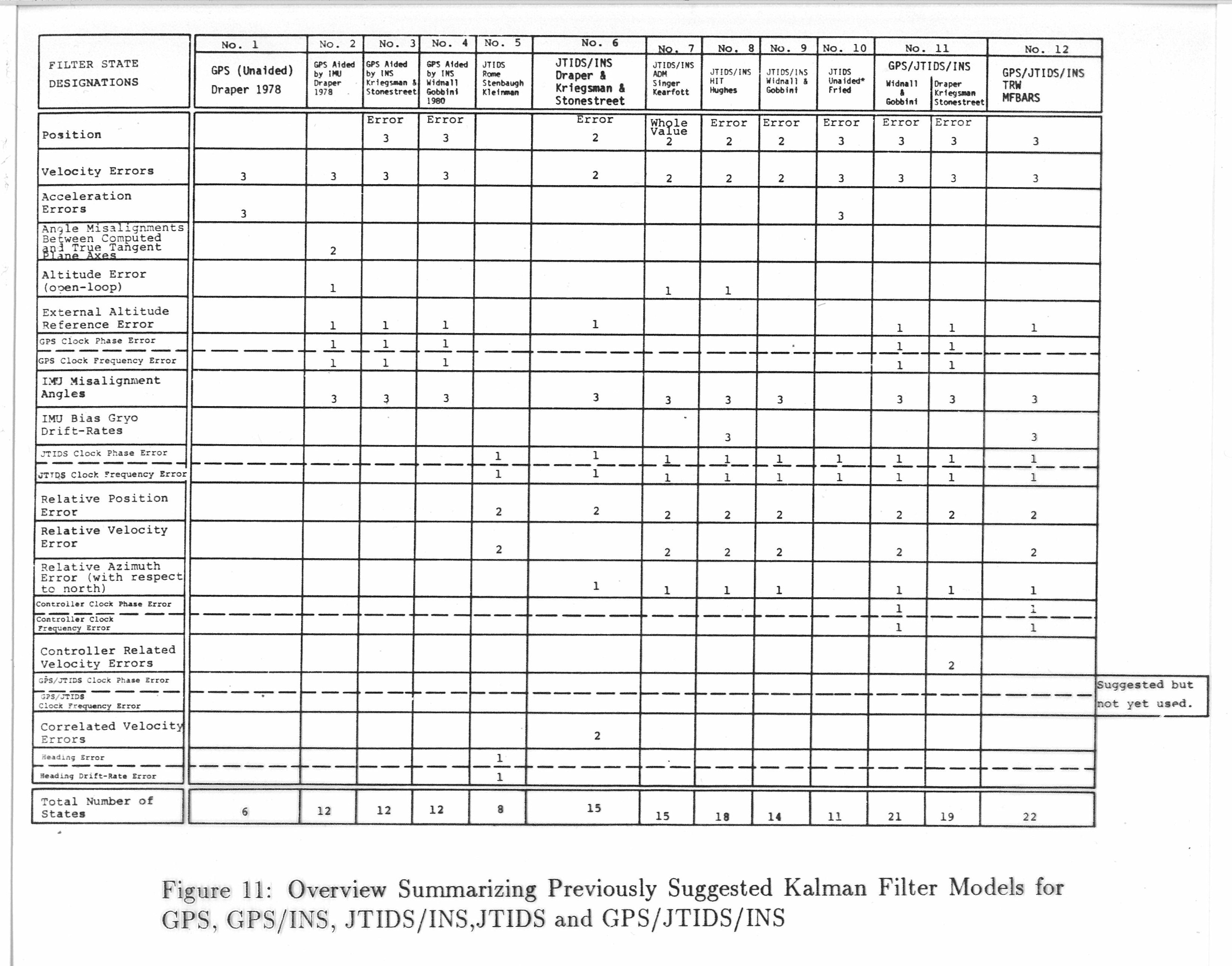
Figure 11 above is identical to Table III (and its explicit reference citations) within: 
Kerr, T. H., “Decentralized Filtering and Redundancy Management for Multi-sensor Navigation,” IEEE Trans. on Aerospace and Electronic Systems, Vol. 23, No. 1, pp. 83-119, Jan. 1987.   (an expose)

Within the MAIN MENU of our TK-MIP GUI, colorization of system blocks appearing in the left margin serves as a gentle visual reminder of which models have already been defined by the USER, corresponding to: System (S), Kalman Filter (KF), and/or resulting Control Gain (M) (if control is present in the application). If control is absent, the corresponding block has no color within the small block diagram in the left margin. Similarly, each block lacks color until it is completely defined enough to proceed in further processing. Such subtle reminders appear on many of our TK-MIP screens throughout.

[One can also accommodate random process mixtures (i.e., the sum) of Gaussian and a small portion of Poison White Noises as a stress test of sorts to determine robustness in the performance of the estimator’s accuracy, as a function of time, when required standard KF and EKF assumptions on the ideal noises “being purely Gaussian” are not strictly met (as determined by User merely introducing a very small amount of corrupting Poison noise). By doing so, User can see if and when the expected performance breaks down and associated estimator accuracy significantly departs from the “design goal” that had been sought.]

This TK-MIP software program utilizes an "n by 1" = (n x 1) discrete-time Linear SYSTEM dynamics of the following form:

(Eq. 1.1)                       x(k+1) = A x(k) + F w(k) + [ B u(k) ],

with

                                      x(0) = x₀ (the initial condition)

and an (m x 1) discrete-time linear Sensor MEASUREMENT (data) observation model of the following algebraic form:

(Eq. 1.2)                       z(k) = C x(k) + G v(k),

where:

                          x(k) is the System State vector at time-step "k",                                   (TK-MIP Requirement is that this is to be USER supplied)

                         A is the (n x n) System Transition Matrix,                                             (TK-MIP Requirement is that this is to be USER supplied)

                          z(k) is the (m x 1) observed sensor data measurement 

                                 vector at time-step "k",                                                                         (TK-MIP Requirement is that this is to be USER supplied)

                          C is the (m x n) Observation Matrix,                                                        (TK-MIP Requirement is that this is to be USER supplied)

                          w(k) & v(k) are INDEPENDENT Gaussian White Noise (GWN) vector sequences with specified variances: Q & R, respectively. 

                          F is the process noise Gain Matrix,                                                           (TK-MIP Requirement is that this is to be USER supplied)

                          G is the measurement noise Gain Matrix,                                                 (TK-MIP Requirement is that this is to be USER supplied)

                          u is an (optional) exogenous control input sequence,                          (TK-MIP Requirement is that this is to be USER supplied, 

                                                                                                                                                     if control is present in application)

                          B is the (optional) Control Gain Matrix for the above control.               (TK-MIP Requirement is that this is to be USER supplied, 

                                                                                                                                                     if control is present in application)

[The above matrices A, C, F, G, B, Q, R can be time-varying explicit functions of the time index "k" or be merely constant matrices. And for the nonlinear case considered further below, it may also be a function of the states, that are replaced by "one time step behind estimates" when an EKF or a 2^nd order EKF is being invoked.] A control, u, in the above System Model may also be used to implement "fix/resets" for navigation applications involving an INS by subtracting off the recent estimate in order to "zero" the corresponding state in the actual physical system at the exact time when the control is applied so that the estimate in both the system and Filter model are both simultaneously zeroed (this is applied to only certain states of importance and not to ALL states). See [95] for further clarification.

In the above discussion, we have NOT yet pinned down or fixed the dimensions of vector processes w(k), v(k), NOR the dimensions of their respective Gain Matrices F, and G here. I am leaving these open for NOW except to say that they will be selected so that the whole of the SYSTEM dynamics equation and algebraic SENSOR data measurements are both properly "conformable" where they occur in matrix addition and matrix multiplication.The open matrix and vector dimensions will be explicitly pinned down in connection with a further discussion of symmetric Q being allowed to be merely positive semi-definite and eventually have a smaller fundamental core (of the lowest possible dimension) that is strictly positive definite for a minimum dimensioned process noise vector. (So further analysis will clear things up and pin down the dimensions to their proper fixed values NEXT!)

See or click on: https://en.wikipedia.org/wiki/Multivariate_normal_distribution#Degenerate_case  [especially see Degenerate Case of prior section]. From Probability and Statistics (topics that we had looked up more than 40 years ago), it is fairly well-known for Gaussians, that if the corresponding covariance 
matrix is only positive semi-definite, then the random variables being considered are linear (more specifically, affine) combinations of the total underlying Gaussians, the number of independent Gaussians present corresponds to the rank of the covariance matrix. The problem can be reduced or simplified to be a consideration of only those fundamental underlying Gaussian variates that are "independent", and their number corresponds to the rank of the original larger Covariance Matrix.The same is true of vector Gaussian radom processes. Likewise, the same is true of the covariances of vector Gaussian white noises.

[For the cases of implementing an Extended Kalman Filter (EKF), or an Iterated EKF, or a Gaussian Second Order Filter (a higher order variant of a EKF that utilizes the first three terms within the multidimensional Taylor Series Expansion {including the 1^st derivative with respect to a vector, being the Jacobian, and the the 2^nd derivative with respect to a vector, being the Hessian}, as obtained outside of TK-MIP, perhaps by hand-calculation) that is being used as a close local approximation to the nonlinear function present on the Right Hand Side (RHS) of the following Ordinary Differential Equation (ODE) representing the system as: 
(Eq. 2.1)  dx/dt = a(x,u,t) + f(x,u,t)w(t) + [ b(x,t)u(t) ],                                                                   (TK-MIP Requirement is that this is to be USER supplied)
(Eq. 2.2)     z(t) = c(x,u,t) + g(x,u,t)v(t)                                                                                          (TK-MIP Requirement is that this is to be USER supplied) 
After the above nonlinear system has been properly linearized by the USER, the resulting matrices A, C, F, G, B, Q, R can be time-varying explicit functions of the time index "k" AND the state "x" AND control "u" (if present) or be merely constant matrices. TK-MIP can also be used to computationally handle this more challenging and more general nonlinear case but estimation results are merely "approximate" (but, perhaps, "good enough") but not "optimal" since the estimates provided via this route are no longer the "conditional expectation of the states, given the measurements" (as required for an "optimal estimator", which, in general, would be intractable in real-time as the important reason or motivation for this necessary trade-off).] 

For Linear Kalman Filters for exclusively linear system models and independent Gaussian Process and Measurement noises, it is fairly straight-forward to handle this situation with only discrete-time filter models, as already addressed above. For similarly handling approximate nonlinear estimation with either an Extended Kalman Filter (EKF) or a Gaussian 2^nd Order Filter, there are three additional steps that must be performed (that we also provide access to the USER within TK-MIP). (1) Step One: Runge-Kutter (R-K) integration of the original nonlinear ODE must be performed between measurements (as a " continuous-time system" with " discrete-time measurement samples" available, as explained in [95]); (2) Step Two: this R-K needs to be applied for the approximate estimator (KF) and for the entire original system [as needed for system to estimator cross-comparisons in determining how well the linear approximate estimator is following the nonlinear state variable "truth model": (3) Step Three: the USER must return to the Database (in defining_model), where the Filter model (KF) was originally entered after the required linearization step had been performed and the results entered. Now everywhere there is a state (e.g., x₁) in the database for the Filter Model, it needs to be replaced by the corresponding estimator result from the previous measurement update step (e.g., xhat₁, respectively). This replacement needs to be performed and completed for every state that appears in the Filter model in implementing either an Extended Kalman Filter (EKF) or in implementing a Gaussian 2nd Order filter. Examples of properly handling these three aspects are offered in: Kerr, T. H., “Streamlining Measurement Iteration for EKF Target Tracking,” IEEE Transactions on Aerospace and Electronic Systems, Vol. 27, No. 2, pp. 408-421, Mar. 1991 and in http://www.dtic.mil/cgi-bin/GetTRDoc?Location=U2&doc=GetTRDoc.pdf&AD=ADP011192.

Insights into the trade-off incurred between magnitude of Q versus magnitude of R as it relates, in simplified form, to the speed-of-convergence of a Kalman filter is offered for a simple scalar numerical example in Sec. 7.1 of Gelb [95]. Recognizing that Q not being positive-definite for the Matrix case is tantamount to "q" being 0 for the scalar case; so let's consider the limiting case as q converges to zero. In particular, Example 7.1-3 for estimating a scalar random walk from a scalar noisy measurement, where the process noise Covariance Intensity Matrix, Q, for this scalar case is "q" and where the measurement noise Covariance Intensity Matrix, R, for this scalar case is "r"; then the resulting steady-state covariance of estimation error is sqrt(rq) and the resulting steady-state Kalman gain is sqrt(q/r). Going further to investigate the behavior of the limiting answer as both q and r become vanishingly small but get there at the same rate of descent, take q = [q'/j²] and take r = [r'/j²], then the resulting steady-state covariance of estimation error is Lim _j-->infinity {[sqrt(r'q')]/j²} = 0  and the resulting steady-state Kalman gain is finite as: Lim _j-->infinity {sqrt(q/r)} = sqrt(q'/r') (a finite non-zero constant) since the j²'s all divide out. Other similar scalar systems in Examples 7.1-4 qnd 7.1-5 again use analytical closed-form results for a Kalman Filter to show the relationship berween convergence and values of "q", "r", and the "time constant" for a first order Markov process.Again, there is dependence on the order of square root in a similar manner but is also an explicit function of the underlying system time-constant as well that is present as an additional term added to the "q" that is present. Examples 7.1-5 and 7.1-6 likewise offer similar insights. Another more comprehensive numerical example offered in Section 7.2  consists of three different design values to be considered for Kalman filter convergence as a function of q, r, and the "time constant" of a first order Markov process. Considering the previous 4 scalar examples from [95] also illustrates why one would never want to have q be identically q = 0 for Kalman Filter applications or else it could be badly behaved or less well-conditioned if not darn right ill-conditioned! These are general principles of Kalman filter convergence behavior as a function of these noise covaiances that have been known for 5 decades (at least since 1974). Reference [95], cited here, is provided on the primary TK-MIP Screen (products).

The white noise w(.):

·         is of zero mean: E [ w(k) ] = 0 for all time steps k,

·         is INDEPENDENT (uncorrelated) as

            E [ w(k) w^T(j) ] = 0 for all k not equal to j (i.e., k ≠  j),

      and as

          E [ w(k) w^T(k) ] = Q for all k,                                                                                                     (TK-MIP Requirement is that this is to be USER supplied)

      where 

           Q = Q^T > 0,        (TK-MIP Requirement is that USER has already verified this property for their application so that estimation within TK-MIP will be well-posed) 

      (i.e., Q = Q^T > 0  above, is standard short notation for Q being a symmetric and positive definite matrix. Please see [71] to [73] and [92] where we, now at TeK Associates, in performing IV&V, historically corrected (all found while under R&D or IV&V contracts during the 1970's and early to mid-1980's) several prevalent problems that existed in the software developed by other organizations for performing numerical verification of matrix positive semi-definiteness in many important DoD applications). Also see http://www2.econ.iastate.edu/classes/econ501/Hallam/documents/Quad_Forms_000.pdf, https://onlinelibrary.wiley.com/doi/pdf/10.1002/9780470173862.app3, References [71] to [73] and [92], cited here, are provided on the primary TK-MIP Screen (i.e., products). Apparently, no better numerical tests are offered within these two more definitive alternate characterizations of positive definiteness and positive semi-definiteness.

·         is Gaussianly distributed [denoted by w(k) ~ N(0,Q) ] at each time-step "k",

·         is INDEPENDENT of the Gaussian initial condition x(0) as: 

            E [ x(0) w^T(k) ] = 0 for all k,

      and is also nominally INDEPENDENT of the Gaussian white measurement noise v(k):

          E [ w(k) v^T(j) ] = 0 for all k not equal to j (i.e., k ≠  j),

      and likewise for the definition of the zero mean measurement noise v(k) 

      except that its variance is R,                                                                                                        (TK-MIP Requirement is that this is to be USER supplied)

      where in the above  

              w^T(·)

      represents the transpose of w(·) and the symbol E [ · ] denotes the standard unconditional expectation operator. 

For estimator initial conditions (i.c.) it is assumed that it is Gaussianly distributed  xhat(t_o) ~ N( x_o, P_o) so that

the initial estimate at time = t_o is:

xhat(t_o)  = x_o,                                                                                                                                  (TK-MIP Requirement is that this is to be USER supplied)

the initial Covariance at time = t_o is:

P(t_o)  = P_o.                                                                                                                                      (TK-MIP Requirement is that this is to be USER supplied)

In the above, the USER (or analyst) usually does not know what true value of x_o to use to get the estimation algorithm started and, similarly, what value of P_o to be used to start the estimation algorithm. The good news is that if the original system and measurement model are “controllable” in the process noise and “observable” in structure, then for the linear case, the Kalman filter is analytically provably to be “exponentially and asymptotically stable” [102], [103] and quickly converges to the correct answer at an exponential rate even if it is started off wrong with an incorrect value for  x_o and an incorrect value for P_o, as long as the starting P_o is "positive definite" (easily achieved if it is taken to be diagonal with all entries positive). Even if the original linear system and measurement model are not controllable and observable, respectively, it will still converge to the correct values reasonably quickly but not as fast as it would if they were controllable and observable. For situations where the original system is NOT “controllable AND observable”, the Kalman filter can still work well but will generally take longer to converge, as a slight inconvenience. The closer the initial guesses or starting values are to the actual but unknown values, the better or faster it will converge to the "right answers" (since the initial guesses are less far away and closer to the ideal situation). References [102], [103], cited here, are provided on the primary TK-MIP Screen (products).

Admittedly, Q-tuning is more prevalent in target tracking applications. For a time-varying Q, it ideally needs to be checked for positive semi-definiteness at each time step. Sometimes such frequent cross-checking is not practicable. An alternative to continuous checking for positive semi-definiteness at each time-step is to provide a "fictitious noise", also known as "Q-tuning", to be positive definite, according to the techniques offered in [82] and [83]. There is also a simple alternative to "Q-tuning" for both the cases of constant and time-varying Q: just by numerically nudging the effective Q to be slightly more "diagonally dominant" as Q_{{modified once}} (k) = Q_{original}(k) + ß· diag[Q_{original}(k)], where diag[Q_{original}(k)] is a diagonal matrix consisting only of the "main diagonal" elements (i.e., top left element to bottom right element) of Q_{original}(k) and all diagonal terms must be positive and the scalar, ß, is a USER specified fixed constant 0 ≤ ß ≤ 1. The theoretical justification for this particular approach to "Q-tuning" is provided by/obtained from Gershgorin disks: https://en.wikipedia.org/wiki/Gershgorin_circle_theorem. "Q-tuning" is, in fact, an Art rather than a Science despite [82] and [83] that attempt to elevate it to the status of a science. Despite what we said earlier above about INS applications usually requiring exact cost accounting, the application for which the "Q-tuning" methodology was developed and applied in [82] involved an airborne INS utilizing GPS within an EKF. Contradictions such as this abound! Implementers will do anything (within reason) to make it work (as well they should)! References [82] and [83], cited here, are provided on the primary TK-MIP Screen (i.e., products). Notice that when the USER makes the scalar ß = 0, then the original Q(k) in the above is unchanged!

Emeritus Prof. Yaakov Bar-Shalom (UCONN), who worked in industry at Systems Control Incorporated (SCI) for many years before joining academia, has many wonderful stories about "Q-tuning" a Kalman tracking filter: in particular, he mentions one application where the pertinent "Q-tuning" was very intuitive but the resulting performance of the Kalman filter was very bad or disappointing and another application, where the "Q-tuning" that he used was counter-intuitive yet the Kalman filter performance was very good. Proper "Q-tuning"  is indeed an art.

Contrasted to the situation for Controllability involving "a controllable pair" (A,B) where all states can be influences by the control effort exerted (which is a good property to possess when seeking to implement a control), while possessing Controllability involving "a controllable pair" (A,F), where all states can be influenced and adversely aggravated by the process noise present (is a bad characteristic to possess). When the underlying systems are linear and time-invariant, the computational numerical tests to verify the above two situations are: rank[B|A·B|A²·B|...|A^(n-1)·B] = n and rank[F|A·F|A²·F|...|A^(n-1)·F] = n, respectively.

Returning to the model, already discussed in detail above (but repeated here again for convenience and for further more detailed analysis), that TK-MIP utilizes as an (n x 1) discrete-time Linear SYSTEM dynamics state variable model of the following form:

(Eq. 3.1)                        x(k+1) = A x(k) + F w(k) + [ B u(k) ], where the process noise w(k) is WGN ~ N(0_n, Q)

with

                                           x(0) = x₀ (the initial condition), where x₀ is from a Gaussian distribution N(x_o, P_o)

and an (m x 1) discrete-time linear Sensor MEASUREMENT (data) observation model of the following algebraic form:

(Eq. 3.2)                            z(k) = C x(k) + G v(k), where the measurement noise v(k) is WGN ~ N(0_m, R);

then, according to Thomas Kailath (emeritus Prof. at Stanford Univ.) that, without any loss of generality, the above model, described in detail earlier above, is equivalent to:

(Eq. 4.1)                        x(k+1) = A x(k) + I_{(n x n)} w(k) + [ B u(k) ], , where the process noise w(k) is distributed as N(0_n, F·Q·F^T); notation: w(k) ~ N(0_n, F·Q·F^T)

with

                                           x(0) = x₀ (the initial condition), where x₀ is from a Gaussian distribution N(x_o, P_o)

and an (m x 1) discrete-time linear Sensor MEASUREMENT (data) observation model is again of the following algebraic form:

(Eq. 4.2)                            z(k) = C x(k) + G v(k), where the measurement noise v(k) is WGN ~ N(0_m, R).

The distinction between the above two model representations is only in the system description, specifically in the Process Noise Gain Matrix, now an Identity matrix, and the associated covariance of the process noise, now having the covariance F·Q·F^T. Such a claim is justified since both representations have the same identical Fokker-Planck equation in common (please see last three pages of [94] explicitly available from this screen below) and consequently, they have the exact same associated Kalman filter when implemented (except for possible minor "tweeks" that can occur in software in possible software author personalization). Reference [94], cited here, is provided on the primary TK-MIP Screen (products).

The prior Measurement noise Controllability Test: rank[F|A·F|A²·F|...|A^(n-1)·F] = n?, respectively. Based on Prof. Thomas Kailath's argument that, without any loss of generality, one can instead focus on F·Q·F^T rather than on Q and F separately in the system dynamics model's description and further factor it into two Cheloski factors, CHELOS, as 

F·Q·F^T = CHOLES*CHOLES^T. Now a more germane test for noise controllability, involving both pertinent parameters of F and Q simultaneously, which now involves checking whether rank[CHOLES|A·CHOLES|A²·CHOLES|...|A^(n-1)·CHOLES] = n?

While possessing a Choleski factorization does serve as a valid test of Matrix positive definiteness and indicates problems being present when it breaks down or fails to go to successful completion when testing a square symmetric matrix for positive definiteness, a drawback is that the number of operations associated with its use is O(n³). There is a version or variation on a direct application of a Choleski decomposition or Choleski factorization known as Aarsen's method that exploits the symmetry of the matrix under test and is only O(n²) in the number of operations required (for testing Q and P ) and O(m²) for testing R_k.

While having a non-positive definite Q-matrix may seem to be a boon by indicating that the process noise does not corrupt all the states of the system in its state variable representation and, similarly, having a non-positive definite R-matrix may be interpreted as being a boon by not all of the measurements being tainted by measurement noise, there can be computational reasons why full rank Q and R are desirable in order to avoid computational difficulties, at least for the standard Kalman filter for the linear case. For the case of long run times, only the so-called SquareRoot Kalman Filter version is "numerically stable" and can tolerate lower rank Q and low rank R without encountering problems with numerical sensitivity.

The availability of “10 Megabyte Ethernet” is a relatively new option for an Input/Output protocol. Since The MathWorks claims that VME is an older protocol that The MathWorks currently (in 2010) doesn’t bother to support, we at TeK Associates are in possession of an Annual Buyer’s guide entitled VME and Critical Systems, Vol. 27, No. 3, December 2009 and we feel obligated to distinguish our TK-MIP software product from that of The MathWorks by TeK Associates eventually offering VME compatibility within TK-MIP in its later versions beyond the current Version 2.0.  

Click here to get the (draft copy) of AIAA Standards for Atmospheric Modeling, as specified by the various U.S. and other International agencies.

Click here to get the (draft copy) of AIAA Standards for Flight Mechanics Modeling, as specified by the pertinent responsible U.S. and other International agencies.

Entries of the requisite matrices, depicted below, can be explicitly numerical (depicted here below as merely constant zeroes: 0.00E+00 throughout) or be in symbolic form consisting of Visual BASIC functions of the independent variable time (or of one of its obvious aliases) and of other parameters and possibly of algebraic operations or combinations (or composites) of such functions. [Entries may also be functions of the specified state variables and of time, as will be evaluated at the prior last available value of the estimate (xhat) or, specifically, xhat at t_minus to allow implementation of Extended Kalman Filters (EKF) or even Gaussian 2^nd Order Filters, as may be needed for particular applications.] Sufficient space is availed within each tabular representation of each entry field. TK-MIP performs the necessary conversions automatically, exactly where they need to occur internal to the TK-MIP software, without the USER needing to explicitly intervene to invoke such conversions themselves. We “do the right thing”, as can be confirmed with copious test problems, using either our favorites, as suggested, or the USER'S own personal favorites. [If this is to be an EKF application for a system that is a nonlinear function of the states (and, possibly also of time and of the exogenous control, u (if present), and the process noise, w, if present), as in Eq. 2.1 dx/dt = a(x,u,t) + f(x,u,t)w(t) + [ b(x,t)u(t) ] above, then it is assumed that the proper entries of the corresponding matrices, such as  A1 here, have already been determined either (i) by manual calculation of the Jacobian matrix, off-line from TK-MIP (since TK-MIP does not offer the capability of performing this calculation within it), or (ii) from some algebraic symbol manipulation program that calculates the Jacobian (i.e., the 1st partial derivative of a[ x(t), u(t), t] with respect to x), for which there are many alternative options outside of TK-MIP for performing this task of obtaining the "Jacobian":

1. Maple Symbolic Math: https://www.maplesoft.com/products/maple/features/symbolicnumericmath.aspx 

2. MapleSim from Maplesoft: https://www.maplesoft.com/products/maplesim/symbolic_computation.aspx 

3. MacSyma: https://en.wikipedia.org/wiki/Macsyma 

4. swMATH MACSYMA: https://www.swmath.org/software/1209 

5. Wolfram Mathematica: https://en.wikipedia.org/wiki/Wolfram_Mathematica 

6. Simplify Calculator: https://www.symbolab.com/solver/simplify-calculator 

7. REDUCE: https://core.ac.uk/download/pdf/82066620.pdf https://reduce-algebra.sourceforge.io/ 

Then upon returning to TK-MIP, the results of the "Jacobian" calculation parameter data is conveyed to TK-MIP as the entries of A1 here. Please notice that such "Jacobian" calculations need be performed only once at the outset but need to be updated as a linearization (reevaluated about the estimate, xhat, obtained from the prior time-step), that must occur within every EKF implementation.]

Aspects of the underlying systems model are entered into a database of the form conveyed below. This facilitates repeated cross-checking of the model that was entered. Appropriate data type conversions are performed so that resulting associated matrices actually used within the calculations are ultimately only floating point, as needed in the actual data processing for underlying Kalman filter processing (and for any of its variations that may have been invoked within TK-MIP for the nonlinear case's approximate estimators) at each crucial time step. For this aspect, it can only work with numerical data for digital implementations (so proper type conversions are mandatory but are done automatically in the background by TK-MIP without USER needing to explicitly intervene).

We utilize database type conversion from (1) strings to (2) functions to (3) double precision floating point numbers, as needed.
Type Conversion Functions (Visual Basic): https://docs.microsoft.com/en-us/dotnet/visual-basic/language-reference/functions/type-conversion-functions  
This data type defines the operations that can be done on the data, the meaning of the data, and the way values of that type can be stored. A data type provides a set of values from which an expression (i.e. variable, function, etc.) may take its values. Runtime Character Type Conversion and Runtime Numeric Type Conversion that are used to an advantage. We convert data types by using OLE Automation Stored Procedures.

Visual Basic provides a means for magnifying each entry within the database cells (corresponding to matrix row and column element entries) so that every aspect of the model is easy to view, enter, cross-check, and thus confirm its correctness. (We will supply the reference for this later; please treat it now as one of TeK Associates' "Trade Secrets".)

Find out what every Microsoft Visual Studio code user needs to know about the GitHub experience:
https://msft.it/6048TWuPo                                                https://channel9.msdn.com/Events/Build/2020/BOD116  

Statisticians (and others working with financial data) appear to be more comfortable with entering system models in this equivalent alternative Auto-Regressive: AR, Auto-Regressive Moving Average: ARMA, or Auto-Regressive Moving Average EXogenous input: ARMAX time-series formulation (to start with) [a preference for going directly to the state variable form may occur later as the User gains more experience and familiarity with it]:

The close (i.e., equivalent) model relationship between a Box-Jenkins time-series representation and a state variable representation has been known for at least  4 or 5 decades, as spelled out in:  A. Gelb (Ed.), Applied Optimal Estimation, MIT Press, Cambridge, MA, 1974. This book also shows how to routinely convert from a discrete-time representation (i.e., involving difference equations) to a continuous-time representation (i.e., involving differential equations) and vice versa. It is the state variable model that is usually used in scientific and engineering applications, where detailed models for the internals of the matrices are available from physical laws that are part of the User's prerequisite academic curriculum or experience. From what I have personally seen in a Data Analytics Conference at Boston University entitled “minnie (Minneapolis) Field Guide to Data Science & Emerging Tech in the Community” on 23 September 2018, they are apparently searching (in the dark in my opinion) for an appropriate black box model in the financial applications areas to use as reasonable models (in conjunction with using parameter estimation and AIC and BIC in order to know when they have a model that adequately captures the essence of the financial application yet the maximum dimension or order stops with a reasonably tractable state-size or AR order-size “n”, as a parameter that appears in the model equations in the image below. In the preceding discussion, the two yet to be defined 3 letter acronyms are: 

Akaike Information Criterion (AIC): https://en.wikipedia.org/wiki/Akaike_information_criterion 


Bayesian Information Criterion (BIC): https://en.wikipedia.org/wiki/Bayesian_information_criterion (It should be no surprise that these two criteria AIC and BIC were used in the same manner as long as 40+ years ago in engineering and scientific applications and in its documented literature.)

In searching for an adequate model for the financial area, It would likely help if Data Scientists followed the work of certain specialists in Econometrics, such as:
1.) Prof.David Luenberger (Stanford University): https://en.wikipedia.org/wiki/David_Luenberger 
2.) (The late) Prof. Monsanao Aoki (UCLA and Univ. of Illinois): https://en.wikipedia.org/wiki/Masanao_Aoki 
3.) Prof. Edison Tse (Stanford University): https://cap.stanford.edu/profiles/frdActionServlet?choiceId=printerprofile&profileversion=full&profileId=41488. 
Each of the above 3 were already extremely well grounded in Modern Control and Estimation theory in the 1960's even before entering into the Econometrics Field. The “Law of Supply and Demand”, “Conspicuous Consumption” and other insights from recognized experts in Macro- and Micro-economics and experienced consultants in various specialty topics should help in these endeavors to capture realistic models for the financial area. Also see: “Special Issue on Stochastic Control methods applied to Financial Engineering,” IEEE Trans. on Automatic Control, Vol. 49, No. 3, Mar. 2004.

Within the MAIN MENU of our TK-MIP GUI, colorization of system blocks in left margin serves as a persistent reminder of which models have been defined by the User, corresponding to: System, Filter, and/or Control (if it is present in the application).

“Gearing up” to complete the modeling, simulation, and implementation tasks, which can all be accomplished much faster by using TK-MIP!