
![]()
![]()
![]()
![]()
![]()
![]()
![]()
![]()
![]()
![]()
![]()
![]()
![]()
![]()
![]()
|
|
|
(Our navigation buttons are at the TOP of each screen.)
Microsoft Word™ is to WordPerfect™ as TK-MIP™ is to ... everything else that claims to perform comparable processing!
Harness the strength and power of a polymath to benefit you! It’s encapsulated within TK-MIP!
Question again: “Who Needs TK-MIP?” Answer: “Anyone with a need to either:..”
The above capabilities of our very USER-centric TK-MIP® should be of high interest to potential customers because:
The graphic image screens
CENTERED sequentially below are representative sample excerpts from
TeK Associates' existing TK-MIP software for
Update: Now 50+ years of experience with Kalman Filter applications and he is an IEEE Life Senior Member and an Associate Fellow of the AIAA in GNC and a Member of SPIE. https://spie.org/profile/Thomas.KerrIII-2982?SSO=1 An option is that the reader may
further pursue any of the underlined topics presented here at their own volition merely by
clicking on the underlined links that follow next. We offer a detailed description
of our stance on use of State Variables and
Descriptor representations and our
strong apprehension concerning use of the Matrix Signum Function and
on
MatLab’s apparent mishandling of Level Crossing situations and our
view of existing problems with certain Random Number Generators (RNG’s)
and other
Potentially Embarrassing Historical Loose Ends further
below. These particular viewpoints motivated the design of our TK-MIP software to avoid these particular problems that we are
aware of and also seek to alert others to. We are cognizant of historical
state-of-the-art software as well [39]-[42].
At General Electric
Corporate Research & Development Center in Schenectady, NY starting in 1971, Dr. Kerr was a protégée of his fellow coworkers: Joe Watson, Hal Moore, Dr. Glenn Roe,
Dean Wheeler, Joel Fleck, Peter Meenan, and Ernie Holtzman within Dr. Richard Shuey's 5046 Industrial Simulations Group performing industrial modeling and computer simulation
and analysis in other computational aspects related to the Automated Dynamic Analyzer (ADA)
continuous-discrete digital simulation of Gaussian white noises as they arise within ODE integration in
feed-forward and feedback loops involving some active but predominately passive elements.
Comment: Dr. Eli Brookner's (Raytheon-retired) book, listed as #14 above, provides its very nice Chapter 3 that is especially helpful in handling the important Kalman filter applications to radar. He not only provides state-of-the-art but also filter state selection designs that were historically relied upon when computer capabilities were more restricted than today and designers were forced to simplify and rely on mere alpha-beta filters (corresponding to position and assumed constant velocity in a Kalman filter in as many dimensions as are actually being considered by the associated radar application: 2-D or 3-D), or on mere alpha-beta-gamma filters (corresponding to position and velocity and assumed constant acceleration in a Kalman filter in as many dimensions as are actually being considered by the associated radar application: 2-D or 3-D). Other historical conventions such as g-h filters or g-h-k filters and common variations such as that of "Benedict-Bordner" are also explained along with their appropriate track initiation. The relation between Kalman filters and Weiner Filters is also addressed, similar to what was provided in [95] (i.e., #6 in the above list). [The above historical perspective is important when the software algorithms present in older hardware are to be upgraded within newer hardware to enable enhanced capabilities.]
#30 as an addendum to the above list: Candy, J. V., Model-Based Signal Processing, Simon Haykin (Editor), IEEE Press and Wiley-Interscience, A John Wiley & Sons, Inc. Publication, Hoboken, NJ, 2006. #31 as an addendum: Bruce P. Gibbs, ADVANCED KALMAN FILTERING, LEAST-SQUARES AND MODELING: A Practical Handbook, John Wiley & Sons, Inc., Hoboken, New Jersey, 2011. #32 as an addendum: Yaakov Bar-Shalom and William Dale Blair (Eds.), Multitarget-Multisensor Tracking: Applications and Advances," Vol. III, Artech House Inc., Boston,
2000. https://ntrs.nasa.gov/api/citations/19770015864/downloads/19770015864.pdf (Yes, Tom Kerr was there in person, as can be verified on page 209 of the attendance list at the end.) For more analytical background perspectives of the entire field, please click on this.
For a system to be Stabilizable [108], those states that are NOT Controllable must decay to 0 anyway. For a system to be Detectable [108], those states that are
NOT Observable must decay to 0 anyway. However, without "Observability and Controllability"
both holding, the rate of convergence of a Kalman Filter is much slower (sometimes
painfully slower)
Please click this for a simple overview perspective.
For more information on the above algorithms, please see [109] and [133].
The numbers computationally obtained are consistent with what has historically first been rigorously proved analytically using proper mathematical analysis and statistical analysis.
TeK Associates® is currently offering a high quality Windowsä 9x\ME\WinNT \2000\XP\Vista\Windows 7\Windows 10 (see Note in Reference [1] within REFERENCES at the bottom of this web page) compatible and intuitive menu-driven PC software product TK-MIP for sale (to professional engineers, scientists, statisticians, and mathematicians and to the students in these respective disciplines) that performs Kalman Filtering for applications possessing linear models and exclusively white Gaussian noises with known covariance statistics (and can perform many alternative approximate nonlinear estimation variants for practically handling nonlinear applications) as well as performing Kalman Smoothing\Monte-Carlo System Simulation and (Optionally) Linear Quadratic Gaussian\Loop Transfer Recovery (LQG\LTR) Optimal Feedback Regulator Control for ONLY the LTI case and which also provides: · Clear on-line tutorials in the supporting theory, including explicit block diagrams describing TK-MIP processing options, · a clear, self-documenting, intuitive Graphical User Interface (GUI). No USER manual is needed. This GUI is easy to learn; hard to forget; and built-in prompting is conveniently at hand as a reminder for the USER who needs to use TK-MIP only intermittently (as, say, with a manager or other multi-disciplinary scientist or engineer). · a synopsis of significant prior applications (with details from our own pioneering experience), · use of Military Grid Coordinates (a.k.a. World Coordinates) for results as well as being in standard Latitude, Longitude, and Elevation coordinates for input and output object and sensor locations, both being available within TK-MIP (for quick and easy conversions back and forth), and for possible inclusion in map output, · implementation considerations and a repertoire of test problems for on-line software calibration\validation, · use of a self-contained on-line consultant feature which includes our own TK-MIP Textbook and also provides answers and solutions to many cutting edge problems in the specific topic areas, · how to access our 1000+ entry bibliography of recent (and historical) critical technological innovations that are included in a searchable database (directly accessible and able to be quickly searched using any derived keyword present in the reference citation, e.g., GPS, author’s name, name of conference or workshop, date, etc.), · option of invoking Jonker-Valgenant-Castanon (J-V-C) algorithm for solving the inherent “Assignment Problem” of Operations Research that arises within Multi-Target Tracking (MTT) utilizing KF-like estimators, · compliance with Department of Defense (DoD) Directive 8100.2 for software, · and manner of effective and efficient TK-MIP® use, so Users can learn and progress at their own rate (or as time allows) with
a quick review always being readily at hand on-line on your own system without having to search for a
misplaced or unintentionally discarded User manual or for an Internet
connection. Besides allowing system simulations for measurement data
generation and its subsequent processing, actual Application
Data can also be processed by TK-MIP,
by accessing sensor data via serial port, via parallel port, or via a variety of commercially
available Data Acquisition Cards (DAQ) using RS-232, PXI,
VXI, GPIB,
Ethernet protocols (as directed by the User) from TK-MIP’s
MAIN MENU. TK-MIP
is independent stand-alone software unrelated to MATLAB®
or SIMULINK®
and, as such, does NOT rely
on or need these products and TK-MIP
RUNS in only
16 Megabytes of RAM. Unfortunately, according to an October 2009 meeting at
The MathWorks, their Data Acquisition Toolbox above currently lacks the ability to handle measurements using the older
VME and PCI protocols, PCI, nor the ability to handle the recent
PCIe protocol. In 2010, the Data Acquisition Toolbox does support
PCIe protocol but still not VME [159].
TeK
Associates believes in being backwards compatible not only in software
but also in hardware and in I/O protocols. Since TK-MIP
outputs its results in an ASCII formatted matrix data stream, these outputs may be passed on
to MATLAB®
or SIMULINK®
after making simple standard accommodations. TeK Associates
is committed to keeping TK-MIP
affordable by holding the price at only $499 for a single User license
(plus $7.00 for Shipping and Handling via regular mail and $15.00 via
FedEx or UPS Blue). TK-MIP software provides screens that prompt the USER on how to configure their system for real-time Data Acquisition:
An ability to perform certain TK-MIP computations for IMM is provided within TK-MIP but doing so in parallel within the framework of Grid Computing is NOT being pursued at this time for two reasons: (1) The a’ priori quantifiable CPU load of this Kalman filter-based variation is modest (as are the CPU burdens of Maximum Likelihood Least Squares-based estimation and LQG/LTR control algorithms as well). (2) Moreover, it has been revealed in 2005 that there is a serious security hole in the SSH (Secure Shell) used by almost all systems currently engaged in grid computing [37]. Multiple
Models of Magill (MMM) and Interactive Multiple Models (IMM) consisting of Banks-of-Kalman-Filters Von Neumann sequential machine
(https://www.britannica.com/technology/von-Neumann-machine,
https://www.geeksforgeeks.org/difference-between-von-neumann-and-harvard-architecture/)
An application example using IMM:
MMM architecture:
Flow charts representative of distinctive aspects of various alternative Multi-target tracking approaches:
IMM architecture:
An example application of Multi-target considerations:
Please click here to view a more recent approach that utilizes Neural Networks to handle some important aspects of Multi-target Tracking. While multi-target tracking in 3-dimentions using
Dynamic Programming was too large a computational burden
TK-MIP
offers pre-specified general structures, with options (already
built-in and tested) that are merely to be User-selected at run time (as
accessed through an easy-to-use logical and intuitive menu structure
that exactly matches this
application technology area). This structure expedites implementation by availing
easy cross-checking via a copyrighted
proprietary methodology [involving proposed software benchmarks of
known closed-form solution, applicable to test any software that
professes to solve these same types of problems] and by requiring less
than a week to accomplish a full scale simulation and evaluation (versus
the 6 weeks to 6 months usually needed to implement from scratch
by $pecialists). USER still has to enter the matrix parameters that characterize or describe their application (an afternoon’s work if they already have this description available, as is frequently the case) Click this link to view the TK-MIP BANNER Screen (and some of its options). To return to this point afterwards to resume reading, merely use the back arrow at the top left of your Web Browser or the keyboard: ALT + Left Arrow. Click this link to view the TK-MIP MAIN MENU screen (and some of its options). To return to this point afterwards to resume reading, merely use the back arrow at the top left of your Web Browser or the keyboard: ALT + Left Arrow. Click this link to view the TK-MIP screen to MATCH S/W TO APP (and some of its alternative processing paths offered within TK-MIP that the USER is to click on to select proper match to their application's structure to that of TK-MIP internal processing without needing to perform any programming themselves). To return to this point afterwards to resume reading, merely use the back arrow at the top left of your Web Browser or the keyboard: ALT + Left Arrow. An
earlier version of TeK Associates’ commercial
software product, TK-MIP Version 1, was unveiled for the first time and
initially demonstrated at our Booth 4304 at IEEE
Electro ’95
in Boston, MA (21-23 June 1995). Our marketing techniques rely on maintaining a
strong presence in the open technical literature by offering new results, new
solutions, and new applications. Since the TK-MIP
Version 2.0 approach allows Users to
quickly perform Kalman Filtering\Smoothing\Simulation\Linear Quadratic
Gaussian\Loop Transfer Recovery (LQG\LTR) Optimal Feedback Regulator
Control, there is
no longer a need for the User to explicitly program these activities
themselves (thus
avoiding any encounters with unpleasant software bugs inadvertently introduced)
and USER may, instead, focus more on the particular application at hand (and its
associated underlying design of experiment). This TK-MIP
software has been validated to also correctly handle time-varying
linear systems, as routinely arise in linearizing general nonlinear systems
occurring in realistic applications. An impressive array of auxiliary supporting
functions are also included within this software such as spreadsheet inputting
and editing of system description matrices; User-selectable color display
plotting on screen and from a printer with a capability to simply specify the
detailed format of output graphs individually and in arrays in order to convey a
story through useful juxta-positioned comparisons; and offering alternative
tabular display of outputs; along with pre-formatted printing of results for ease-of-use and clarity by pre-engineered design; automatic
conversion from continuous-time state variable or auto-regressive (AR) or
auto-regressive moving average (ARMA) mathematical model system representation
to discrete-time state variable representation [95]
(i.e., as a Linear System
Realization); facilities for simulating vector colored noise of
specified character rather than just conventional white noise (by providing the
capability to perform Matrix
Spectral Factorization (MSF) to obtain the requisite preliminary shaping
filter). [These last two features are only
found in TK-MIP
to date. There is more on MSF to follow next below.] Another
advantage possessed by TK-MIP®
over any of
our competitor’s
software is that we provide the only software that successfully implements
Matrix Spectral Factorization (MSF) as a precedent. MSF is a Kalman Filtering
accoutrement that enables the rigorous routine handling (or system modeling) of
serially time-correlated measurement noises and process noises that would
otherwise be too general and more challenging than could normally be handled
within a standard Kalman filter framework that expects only additive Gaussian
White Noise (GWN) as input. Such unruly, more general noises are
accommodated within TK-MIP via a two-step procedure of (1) using MSF
to decompose them into an associated dynamical system Multi-Input Multi-Output (MIMO)
transfer function ultimately stimulated by (WGN) and then (2) our
explicitly implementing an algorithm for specifying a corresponding linear
system realization representing the particular specified MIMO
time-correlation matrix or, equivalently, its power spectral matrix. Such
systems structurally decomposed in this way can still be handled or processed
now within a standard estimation theory framework by just increasing the
original systems dimension by augmenting these noise dynamics into the known
dynamics of the original system, and then both can be handled within a standard state-variable
or descriptor system formulation of somewhat higher dimensions. These
techniques are discussed and demonstrated in:
A
more realistically detailed model may be used for the system
simulation while alternative reduced-order models can be used for
estimation and\or control, as usually occurs in practice because of
constraints on tolerable computational delay and computational
capacity of supporting processing resources, which usually restricts
the fidelity of the model to be used in practical implementations to
principal components that hopefully “capture the essence” of the
true system behavior. Simulated noise in TK-MIP
can be Gaussian white noise, Poisson white noise (but not usually and almost
never), or a weighted
mixture of the two (with specified variances being provided for both
as User-specified inputs) as a worse case consideration in a
sensitivity evaluation of application designs. Filtering and\or
control performance sensitivities may also be revealed under
variations in underlying statistics, initial conditions, and
variations in model structure, in model order, or in its specific
parameter values. Prior to pursuing the above described detailed
activities, Observability\Controllability
testing can be performed automatically (for linear time-invariant
applications) to assure that structural conditions are suitable for performing Kalman filtering, smoothing, and optimal control. A novel aspect is that there is a
full on-line tutorial on how to use the software as well as describing
the theoretical underpinnings, along with block diagrams and
explanatory equations since TK-MIP
is also designed for the novice
student Users from various disciplines as
well as for experts in electrical or mechanical engineering, where
these techniques originated. The pedagogical detail may be turned off (and is automatically unloaded from RAM during actual signal
processing so
that it doesn’t contribute to any unnecessary overhead) but may be turned back on
any time a gentle reminder
is again sought. A sophisticated proprietary pedagogical technique is
used that is much more responsive to immediate USER questions than
would otherwise be availed by merely interrogating a standard WINDOWS 9X/2000/ME/NT/XP Help system and this is enhanced by exhibiting descriptive equations
when appropriate for knowledgeable Users. TK-MIP
also includes the option of activating a modern
version of square root Kalman filtering (for effectively achieving
double precision accuracy without actually invoking double precision
calculations nor incurring additional time delay overhead beyond what is
present for a standard version of Kalman filtering) which is a
numerically stable version for real-time on-line use, that provides a
software architecture for benignly handling round-off, where this type
of robustness is important over the long haul of continuous real-time operation. TK-MIP provides clear insightful explainations of underlying theorectical aspects involving both implementation and statistical
Additional discussion of the class of Alpha-stable filters mentioned above: Simulation Demos at earlier IEEE Electro: Although the TK-MIP software is general purpose, TeK Associates originally demonstrated this software in Boston, MA on 21-23 June 1995 for (1) the situation of an aircraft equipped with an Inertial Navigation System (INS) using a Global Positioning System (GPS) receiver for periodic NAV updates;(2) several benchmark test problems of known closed-form solution (for comparison purposes in verification\validation). These are both now included within the package as standard examples to help familiarize new Users with the workings of TK-MIP. This TK-MIP software program utilizes an (n x 1) discrete-time Linear SYSTEM dynamics state variable model of the following form: (Eq. 1.1) x(k+1) = A x(k) + F w(k) + [ B u(k) ], with x(0) = x0 (the initial condition) and an (m x 1) discrete-time linear Sensor MEASUREMENT (data) observation model of the following algebraic form: (Eq. 1.2) z(k) = C x(k) + G v(k),
[The above matrices A, C, F, G, B, Q, R can be time-varying explicit functions of the time index "k" or be merely constant matrices. And for the nonlinear case considered further below, these matrices may also be a function of the states (that are later eventually replaced in the FILTER Model by "one time-step behind estimates" when an EKF or a 2nd order EKF is being invoked).] A control, u, in the above System Model may also be used to implement "fix/resets" for navigation applications involving an INS by subtracting off the recent estimate in order to "zero" the corresponding state in the actual physical system at the exact time when the control is applied so that the estimate in both the system and Filter model are both simultaneously zeroed (this is applied to only certain states of importance and not to ALL states). See [95] for further clarification. In the above discussion, we have NOT yet pinned down or fixed the dimensions of vector processes w(k), v(k), NOR the dimensions of their respective Gain Matrices F, and G here. I am leaving these open for NOW except to say that they will be selected so that the whole of the SYSTEM dynamics equation and algebraic SENSOR data measurements are both properly "conformable" where they occur in matrix addition and matrix multiplication. The open matrix and vector dimensions will be explicitly pinned down in connection with a further discussion of symmetric Q being allowed to be merely positive semi-definite and eventually have a smaller fundamental core (of the lowest possible dimension) that is strictly positive definite for a minimum dimensioned process noise vector. (So further analysis will clear things up and pin down the dimensions to their proper fixed values NEXT!) See or click on: https://en.wikipedia.org/wiki/Multivariate_normal_distribution#Degenerate_case
[Especially see Degenerate Case of section just prior.] [For the cases of implementing an Extended Kalman Filter
(EKF), or an Iterated EKF, or a Gaussian Second Order Filter (a higher order variant of a EKF that utilizes the first three terms within the
multidimensional Taylor Series Expansion {including the 1st
derivative with respect to a vector, being the Jacobian, and the the 2nd
derivative with respect to a vector, being the Hessian}, as obtained outside of
TK-MIP, perhaps by hand-calculation) that is being used as a close local approximation to
the nonlinear function present on the Right Hand Side (RHS)
of the following Ordinary Differential Equation (ODE)
representing the system as: For Linear Kalman Filters for exclusively linear system models and independent Gaussian Process and Measurement noises, it is fairly straight-forward to handle this situation with only discrete-time filter models, as already addressed above. For similarly handling approximate nonlinear estimation with either an Extended Kalman Filter (EKF) or a Gaussian 2nd Order Filter, there are three additional steps that must be performed (that we also provide access to the USER within TK-MIP). (1) Step One: A Runge-Kutta (RK) 4(5) or, preferably, a Runge-Kutta-Fehlberg 4(5) method, with automatically adaptive step-size https://maths.cnam.fr/IMG/pdf/RungeKuttaFehlbergProof.pdf integration of the original nonlinear ODE must be performed between measurements (as a " continuous-time system" with " discrete-time measurement samples" available, as explained in [95]); (2) Step Two: this R-K needs to be applied for the approximate estimator (KF) and for the entire original system [as needed for system to estimator cross-comparisons in determining how well the linear approximate estimator is following the nonlinear state variable "truth model": (3) Step Three: the USER must return to the Database (in defining_model), where the Filter model (KF) was originally entered after the required linearization step had been performed and the results entered. Now everywhere there is a state (e.g., x1) in the database for the Filter Model, it needs to be replaced by the corresponding estimator result from the previous measurement update step (e.g., xhat1, respectively). This replacement needs to be performed and completed for every state that appears in the Filter model in implementing either an Extended Kalman Filter (EKF) or in implementing a Gaussian 2nd Order filter. Examples of properly handling these three aspects are offered in: .Kerr, T. H., “Streamlining Measurement Iteration for EKF Target Tracking,” IEEE Transactions on Aerospace and Electronic Systems, Vol. 27, No. 2, pp. 408-421, Mar. 1991 and in http://www.dtic.mil/cgi-bin/GetTRDoc?Location=U2&doc=GetTRDoc.pdf&AD=ADP011192. Insights into the trade-off incurred between magnitude of
Q versus magnitude of R as it relates, in simplified form, to the speed of convergence of a Kalman filter is
offered for a simple scalar numerical example in Sec. 7.1 of Gelb [95].
Consider that Q not being positive definite for the Matrix case is
tantamount to q being zero for the scalar case; so let's consider the
limiting case as q converges to zero. In particular,
Example 7.1-3 for estimating a scalar random walk from a scalar noisy
measurement, where the process noise Covariance Intensity Matrix, Q, for this scalar case is
"q" and where the measurement noise Covariance Intensity Matrix,
R, for this scalar case is "r"; then the resulting steady-state covariance of estimation error is
sqrt(rq) and the resulting steady-state Kalman gain is sqrt(q/r). Going further to investigate the behavior
of the limiting answer as both
q and r become vanishingly small, take q = [q'/j2]
and take r = [r'/j2], then the resulting steady-state covariance of estimation error is
Lim j→∞ {[sqrt(rq)]/j2}
= 0 (since the j2's all divide out) and the resulting steady-state Kalman gain is finite as:
Lim j→∞
{sqrt(q/r)} = sqrt(q'/r')
(a finite constant). Another numerical example offered as Sec. 7.1-4 is three
different design values to be cxonsidered for Kalman filter convergence as a
function of q, r, and the time constant of a first order Markov process. These
are general principles of Kalman filter convergence behavior as a function of
these noise covariances that have been known for
5 decades. A clearer exhibition of the effect of "Q" and "R" (or scalar
"q" and scalar "r", respectively) on the convergence of a simplified 2-state Kalman filter (for illustrative purposes) is conveyed in: The white noise w(.): · is of zero mean: E [ w(k) ] = 0 for all time steps k, · is INDEPENDENT (uncorrelated) as E [ w(k) wT(j) ] = 0 for all k not equal to j (i.e., k ≠ j), and as E [ w(k) wT(k) ] = Q for all k, (TK-MIP Requirement is that this is to be USER supplied) where Q = QT > 0, (TK-MIP Requirement is that USER has already verified this property for their application so that estimation within TK-MIP will be well-posed) (i.e.,
Q = QT > 0 above, is standard short notation for
Q being a symmetric and positive definite matrix. Please see
[71] to [73]
and [92] where we, now at TeK Associates,
in performing IV&V, historically corrected (all found while under R&D or
IV&V contracts
during the 1970's and early to mid-1980's) several prevalent problems that existed in
the software developed by other organizations for performing numerical verification of matrix
positive semi-definiteness (and positive definiteness) in many important DoD applications). Also see http://www2.econ.iastate.edu/classes/econ501/Hallam/documents/Quad_Forms_000.pdf,
https://onlinelibrary.wiley.com/doi/pdf/10.1002/9780470173862.app3. Apparently, no better numerical tests are offered within these two more
recent and definitive alternate characterizations of positive definiteness and positive
semi-definiteness yet, thankfully, others are still trying: see New insights into matrix semi-definiteness:
https://mjo.osborne.economics.utoronto.ca/index.php/tutorial/index/1/qfs/t. · is Gaussianly distributed [denoted by w(k) ~ N(0,Q) ] at each time-step "k", · is INDEPENDENT of the Gaussian initial condition x(0) as: E [ x(0) wT(k) ] = 0 for all k, and is also nominally INDEPENDENT of the Gaussian white measurement noise v(k): E [ w(k) vT(j) ] = 0 for all k not equal to j (i.e., k ≠ j), and likewise for the definition of the zero mean measurement noise v(k) except that its variance is R, (TK-MIP Requirement is that this is to be USER supplied) where in the above wT(·) represents the transpose of w(·) and the symbol E [ · ] denotes the standard unconditional expectation operator. For estimator initial conditions (i.c.'s), it is assumed that
it is Gaussianly distributed as N(
xo, Po) so that the initial estimate at time =
to is: xhat(to) =
xo,
(TK-MIP Requirement is that this is to be USER supplied) the initial Covariance at time =
to is: P(to) = Po. (TK-MIP Requirement is that this is to be USER supplied) In the above, the USER (or analyst) usually does not
know what true value of
xo to use to get the estimation algorithm started and, similarly, what
value of Po to
be used to start the estimation algorithm. The good news is that
if For applications involving very accurate Inertial Navigation Systems (INS), as for U.S. SSBN's and SSN's for example, it is usually the case that one only uses the exact values that have been determined for Q (after laborious calibration on a test stand, perhaps by others). Values used for Q in these types of INS applications are like accounting problems that seek exactness in the values used. These values are assumed to have already passed some earlier off-line positive definiteness test or else they would have never gotten so far as to be documented for subsequent data entry for this type of application. Admittedly, Q-tuning is more prevalent in target tracking applications. For a time-varying Q(k), it may ideally need to be checked for positive semi-definiteness/positive definiteness at each time step. Sometimes such frequent cross-checking is not practicable. An alternative to continuous checking for positive semi-definiteness at each time-step is to provide a "fictitious noise", also known as "Q-tuning", to be positive definite, according to the techniques offered in [82] and [83]. There is also a simple alternative to "Q-tuning" for both the cases of constant and time-varying Q: just by numerically nudging the effective Q to be slightly more "diagonally dominant" as Q{modified once}(k)= Q{original}(k)+ ß· diag[Q{original}(k)], where diag[Q{original}(k)] is a diagonal matrix consisting only of the "main diagonal" (i.e., top left element to bottom right element) of Q{original}(k) and all diagonal terms must be positive and the scalar, ß, is a USER specified fixed constant 0 ≤ ß ≤ 1. The theoretical justification for this particular approach to "Q-tuning" is provided by/obtained from Gershgorin disks: https://en.wikipedia.org/wiki/Gershgorin_circle_theorem. "Q-tuning" is, in fact, an Art rather than a Science despite [82] and [83] that attempt to elevate it to the status of a science. Despite what we said earlier above about INS applications usually requiring exact cost accounting, the application for which the "Q-tuning" methodology was developed and applied in [82] involved an airborne INS utilizing GPS within an EKF. Contradictions such as this abound! Implementers will do anything (within reason) to make it work (as well they should)! In particular, notice that when the USER makes the scalar ß = 0, then the original Q in the above is unchanged! Emeritus Prof. Yaakov Bar-Shalom (UCONN), who worked in industry at Systems Control Incorporated (SCI) in Palo Alto, CA for many years before joining academia, has many wonderful stories about "Q-tuning" a Kalman tracking filter: in particular, he mentions one application where the pertinent Q-tuning was very intuitive but the resulting performance of the Kalman filter was very bad or disappointing and another application, where the Q-tuning that he used was counter-intuitive yet the Kalman filter performance was very good. Proper Q-tuning is indeed an art. Contrasted to the situation for Controllability involving "a controllable pair"
(A,B) where all states can be influences
by the control effort exerted (which is a good property to possess when seeking to implement a
control), while
possessing Controllability involving "a controllable pair" (A,F), where all states can be influenced
and adversely aggravated by the process noise present (is a bad characteristic to
possess). When the underlying systems are linear and time-invariant, the
computational numerical tests to verify the above two situations are: rank[B|A·B|A2·B|...|A(n-1)·B] = n
and rank[F|A·F|A2·F|...|A(n-1)·F] = n, respectively. The
augmented matrices that were checked to see if they had rank = n (the dimension of the state) are Called the Controllability Grammian. A corresponding augmented matrix involves transposes throughout and is called the
"Observability Grammian". “Observability”
and "Controllability” yea/nay tests for linear systems with time-varying “System
matrix”, “Obsevation matrix”, and “System Noise Gain matrix” are presented in
[59], as developed by Leonard
Silverman, but are difficult to implement for a general time-varying case; so it
is not used within TK-MIP. If desired, a USER may perform their own specialized investigation using this controllability test to satisfy their own suspicions regarding a
proper answer. Over a short enough time-step, system structure and parameter
values are essentially CONSTANT. For discrete-time sample value systems, answers to these types of questions are available within "n" time-steps, where "n" is the dimension or state-size of the system being investigated. Returning to the model, already discussed in detail above (but repeated here again for convenience and for further more detailed analysis), that TK-MIP utilizes as an (n x 1) discrete-time Linear SYSTEM dynamics state variable model of the following form: (Eq. 3.1) x(k+1) = A x(k) + F w(k) + [ B u(k) ], where the process noise w(k) is WGN ~ N(0n, Q) with x(0) = x0 (the initial condition), where x0 is from a Gaussian distribution N(xo, Po) and an (m x 1) discrete-time linear Sensor MEASUREMENT (data) observation model of the following algebraic form: (Eq. 3.2) z(k) = C x(k) + G v(k), where the measurement noise v(k) is WGN ~ N(0m, R); then, according to Thomas Kailath (emeritus Prof. at Stanford Univ.) that, without any loss of generality, the above model, described in detail earlier above, is equivalent to: (Eq. 4.1) x(k+1) = A x(k) + I(n x n) w(k) + [ B u(k) ], with identity matrix I(n x n) and process noise w(k) distributed as N(0n, F·Q·FT); notation: w(k) ~ N(0n, F·Q·FT) with x(0) = x0 (the initial condition), where x0 is from a Gaussian distribution N(xo, Po) and an (m x 1) discrete-time linear Sensor MEASUREMENT (data) observation model is again of the following algebraic form: (Eq. 4.2) z(k) = C x(k) + G v(k), where the measurement noise v(k) is WGN ~ N(0m, R). The distinction between the above two model representations is only in the system description, specifically in the Process Noise Gain Matrix, now an Identity matrix, and the associated covariance of the process noise, now having the covariance F·Q·FT. Such a claim is justified since both representations have the same identical Fokker-Planck equation in common (please see Appendix 4 in [124] or last three pages of [94] explicitly available from this screen below) and consequently, they have the exact same associated Kalman filter when implemented (except for possible minor "tweeks" that can occur in software within possible software author personalization).
F·Q·FT = CHOLES·CHOLEST. Now a more germane test for noise controllability, involving both pertinent parameters of F and Q simultaneously, which now involves checking whether rank[CHOLES|A·CHOLES|A2·CHOLES|...|A(n-1)·CHOLES] = n? While possessing a Cholesky (http://www.math.utoledo.edu/~codenth/Linear_Algebra/Calculators/Cholesky_factorization.html) does serve as a valid test of Matrix positive definiteness and indicates problems being present when it breaks down or fails to go to successful completion when testing a square symmetric matrix for positive definiteness, a drawback is that the number of operations associated with its use is O(n3). There is a version or variation on a direct application of a SVD (already declared by others as the best method for determining or revealing a matrix's definiteness, semi-definiteness, or lack thereof) known as "Aarsen's method" [92] that exploits the symmetry of the matrix under test to an advantage and is only O(n3), but lower at n3/6, in the number of operations required (for testing Q and P ) and O(m3) for testing R. By way of comparison, the QR Algorithm for symmetric matrices requires O(n2) operations per step [109, p. 414] for n steps so still O(n3) in total. While having a non-positive definite Q-matrix may seem to be a boon by indicating that the process noise does not corrupt all the states of the system in its state variable representation and, similarly, having a non-positive definite R-matrix may be interpreted as being a boon by not all of the measurements being tainted by measurement noise, there can be computational reasons why full rank Q and R are desirable in order to avoid computational difficulties, at least for the standard Kalman filter for the linear case. For the case of long run times, only the so-called Squareroot Kalman Filter version is "numerically stable" and can tolerate lower rank Q and low rank R without encountering problems with numerical sensitivity. SAVING THE BEST FOR LAST: Frequently, "Q-tuning" is invoked when using a reduced-order filter for an application that has a much larger dimensioned "Truth model". The underlying idea being that one attempts to capture the essence of the application's behavior (as in an approach to identifying the "Principal Components", which describe the essential behavior of the underlying system) with the reduced-order (lower-order) filter model utilized. Then one makes use of fictitious "Q-tuning" to approximately account for the "unmodeled dynamics" NOT explicitly included in the reduced-order "filter model". Sometimes, the approximate model resorted to is essentially a WAG (i.e., an outright "Wild Ass Guess", please excuse my use of this well-known expression in this context). Surprisingly, this frame work just described can be somewhat forgiving as long as it is guided by good engineering insight and a diligent attempt to capture the pertinent (and prominent) system behavior and characteristics. A numerical example to put various dimensions for a particular reduced-order Kalman filter in perspective follows next. For U.S. Poseidon SSBN's some fifty years ago [106], Sperry Systems Management (SSM) in Great Neck, NY had established a detailed error model for the G-7B INS, a conventional 3-input axis spinning rotor gyro: it's detailed error (Truth) model consisted of 34 states. It's associated Kalman Filter model consisted of only 7 states and was called the 7-State STAtistical Reset Filter (STAR filter). Also see page 282 of [115]. (The identities of these states are not divulged in either references [106] or [115].) Thanks to the empirical Moore's Law since 1965 and into the near future, medium future, and far future, trends in available computer resources to support implementation of Kalman filters and their respective system and measurement models are considerably less constraining and consequently now tolerate more detailed larger dimensional models conveying a more accurate representation of the application system and measurement structure.
The importance or impact of symmetric matrices being positive definite versus being merely positive semi-definite can best be understood by considering their impact on the corresponding "quadratic forms" involving these symmetric matrices. For y = xTQx, taking Rn into R1, the shape of the paraboloid is "strictly convex" and y is positive for all x ≠ 0, while for a matrix Q that is positive semi-definite, there is no longer guaranteed convexity and there can be some flatness in the associated paraboloid when y is used as a "cost function". Having convex cost functions is useful when attempting to intersect regions of interest so that the results will be well-behaved and not pathological. Such issues arise in minimum energy Linear Quadratic Optimal Control regulators for both Finite Planning Horizons (integrating the two term integrand:∫oτ [xT(t)Q(t)x(t) + uT(t)R(t)u(t)] dt (with respect to time) from 0 to finite positive τ) and for Infinite Planning Horizons (integrating the two term integrand: ∫o∞ [xT(t)Qx(t) + uT(t)Ru(t)]dt (with respect to time, from 0 to infinity: ∞). The correspondingly appropriate existing constraint is that the system dynamics is described by a linear Ordinary Differential Equation (ODE) of the standard form dx/dt = Ax(t) + Bu(t), where the control, u(t), is to be determined to minimize the two term cost functions previously presented and to have the feedback form u(t) = GAIN·[x(t) - z(t)] = GAIN· [In x n - C] x(t). Indeed, there is a long recognized "duality" between the Optimal Linear Quadratic Regulator problem and the Linear Kalman Optimal Filter problem (see Blackmore, P. A., Bitmead, R. R., “Duality Between the Discrete-Time Kalman Filter and LQ Control Law,” IEEE Transactions on Automatic Control, Vol. AC-40, No. 8, pp. 1442-1443, Aug. 1995). Also see [70], where we discuss even more Kalman Filter applications): both involve calculating the proper gain matrix to use and both involve solving a Riccati equation to obtain the proper gain matrix. A Riccati equation is to be solved forwards in time for the Kalman Filter while another Riccati equation is to be solved backwards in time for the minimum energy Linear Quadratic Regulator. Other applications where convex functions over convex regions are beneficial in further analysis in order that the results be analytically well-behaved are provided by us in [110] - [116] (please see [117] - [123], [127] for further independent confirmation/substantiation by others of the usefulness of convex functions and convex sets in this way within the field of engineering and optimization). For both the "Finite Planning Horizon" and the "Infinite Planning Horizon", the R and Q appearing within the corresponding integral cost functions, respectively, are still symmetric and positive definite but are NOT covariance intensity matrices, as defined following Eqs. 1.1, 1.2, 2.1, 2.2, 3.1, 3.2, 4.1,4.2 but play a similar role in the corresponding associated Riccati Equations, since the linear "quadratic regulator" control problem is the mathematical "dual" of the linear filtering problem, as originally recognized by Rudolf Kalman back in the 1960's when he correctly posed and solved both using similar techniques with similar resulting solution structure.
The image below portrays the delineation between the structural situations for those applications that warrant use of a Luenberger Observer (LO) and those that warrant use of a Kalman Filter (KF) and the "regularity conditions" that support its use for applications of state estimation and/or additionally Linear Quadratic (LQ) Minimum Energy Control. Easily accessible explanations of LO are available in [9], [99], [100].
These prior definitions above are repeated again within the section on "Defining Model(s)" as a convenient refresher for the USER closer to the discussion where it is to be performed by the USER as "actionable" in modern business parlance. The following more concise discussion is from actual screen shots of TK-MIP: which also defines the pertinent vector and matrix dimensions:
Notice in the above screen shot that possible correlation between the process noise and the measurement noise is acknowledged. When that occurs, instead of the Kalman Gain being: Eq. 4.3 Kk = Pk|k-1CkT [CkPk|k-1CkT + Rk]-1, it then becomes Eq. 4.4 Kk = Pk|k-1CkT [CkPk|k-1CkT + Sk + Rk]-1 [107], where, in the above, matrix Sk is the conformable correlation Matrix between GWN process noise and GWN measurement noise (denoted by [ QR ] in the above image). While there is an algorithm known as the QR algorithm, the above is NOT referencing the QR algorithm but is merely notation for the pertinent cross-correlation that may exist in some applications between process noise and measurement noise. Apparently, the previous simple summarizing expression is only possible when the dimension of the system (or plant) noise is identical to the dimension of the measurement or sensor noise (not a very realistic situation in most applications). Examples of practical engineering situations where such structures may be useful are: (1) for INS-stabilized missiles, drones, and UAVs that may use occasional or periodic external position fixes, wind buffeting may affect INS System model noise intensity that may then directly adversely affect lever arm positioning of external positioning sensor (with respect to their center-of-gravity) as it makes use of the external measurements to compensate for INS build-up of gyro-drift; (2) on a U-2 (or, perhaps, by now, on a U-3) that seeks to use INS-pointing to take simultaneous multi-sensor images in order to triangulate or get a visual position fix enroot. Upon inserting the above modified sequence for the Kalman Gain Kk that includes Sk within the well-known Joseph Form for the Covariance of Estimation Error update equation, according to the tenets of standard Covariance Analysis when determining an Error Budget, one obtains the correct Covariance of Error associated with this now modified Kalman Gain matrix that includes the cross-correlation Sk between System and Measurement noises. Also see: Y. Sunahara, A. Ohsumi, K. Terashima, H. Akashi, "Representation of Solutions and Stability of Linear Differential Equations with Random Coefficients via Lie Algebraic Theory," 11th JAACE Symposium on Stochastic Systems, Kyoto, pp. 45-48, 27-29 Nov. 1979.
My earliest extensive Kalman filter modeling was for a ship-borne
Inertial Navigation System (INS) that was aided by using a variety of alternative
"navaids" for
Now, simulation studies can be performed to cross-compare resulting INS accuracies
in a variety of application scenarios as a function of time and "navaid" usage at
For radar target tracking applications, what is modeled within the Kalman Filter
is the dynamics behavior of the designated target. In seeking to intercept an enemy In pursuing radar applications, it is advisable to first get a nice overview by reading the following book: https://thesource2.metro.net/i/document/K0W1U2/radar-principles-for-the-nonspecialist_pdf https://digital-library.theiet.org/content/books/ra/sbra032e Personally, I try to keep abreast of nice new discussions or revelations in radar: https://us.artechhouse.com/Radar-for-Fully-Autonomous-Driving-P2262.aspx (This new book is highly recommended for what it contains!) https://hal.archives-ouvertes.fr/hal-01070959/document https://www.facebook.com/IEEEAESS/videos/passive-radar/748838592565039/ For aircraft and other air-borne or space-borne radar targets, it is important to know the effect of fluctuations, as contained in information regarding
Useful tools for handling actual data for the application: Julian-to-local-time conversions and Calendar conversions.
Elaborating further on TK-MIP Version 2.0 CURRENT CAPABILITIES: This Software package allows/enables the USER to: ·
SIMULATE any Gauss-Markov process specified in linear time-invariant (or time-varying) state space form of arbitrary dimension N (usually N is less than 200 and frequently much less). · TEST for WHITENESS and NORMALITY of SIMULATED Gaussian White Noise (GWN) sequence: w(k) for k=1, 2, 3,... (ultimately from underlying Pseudo-Random Number [PRN] generator). · SIMULATE sensor observation data as the sum of a Gauss-Markov process, C x(k), and an INDEPENDENT Gaussian White Measurement Noise, G v(k). · DESIGN and RUN a Kalman FILTER with specified gains, constant or propagated, on REAL (Actual) or SIMULATED observed sensor measurement data. · DESIGN and RUN a Kalman SMOOTHER (now also known as Retro-diction) or a Maximum Likelihood Batch Least Squares algorithm on REAL (actual) or SIMULATED data. · DISPLAY both DATA and ESTIMATES graphically in COLOR and\or output to a printer or to a file (in ASCII). · CALCULATE SIMULATOR and ESTIMATOR response to ANY (Optional) Control Input. · EXHIBIT the behavior of the Error Propagation (Riccati) Equation: · For full generality, unlike most other Kalman filter software packages or add-ons like MATLAB® with SIMULINK® and their associated Control Systems toolkit, TK-MIP avoids using Schur computational techniques, which are only applicable to a narrowly restricted set of time-invariant system matrices and TK-MIP® also avoids invoking the Matrix Signum function for any calculations because they routinely fail for marginally stable systems (a condition which is not usually warned of prior to invoking such calculations within MATLAB®). See Notes in Reference [2] at the bottom of this web page for more perspective. · From a current session either the final result or incremental intermediate result having just been completed, USER can SAVE-ALL at END of each Major Step (to gracefully accommodate any external interruptions imposed upon the USER) or RESURRECT-ALL results previously saved earlier, even from prior sessions. [This feature is only available for the simpler situation of having linear time-invariant (LTI) models and not for time-varying models, nor for nonlinear situations, nor for Interactive Multiple Model (IMM) filtering situations, all of which can be handled within TK-MIP after slight modifications (as directed by the USER from the MAIN MENU, Model Specification, and Filter Processing screens) but these more challenging scenarios do NOT offer the SAVE-ALL and RESURRECT-ALL capability because of the additional layers of complexity to be encountered for these special cases causing them to be less amenable to being handled within a single structural form]. · OFFER EXACT discrete-time EQUIVALENT to continuous-time white noise (as a USER option) for greater accuracy in SIMULATION (and closer agreement between underlying model representation in FILTERING and SMOOTHING). · AVAIL the USER with special TEST PROBLEMS\TEST CASES (of known closed-form solution) to confirm PROPER PERFORMANCE of any software of this type. · OFFER ACCESS to time histories of User-designated Kalman Filter\Smoother COVARIANCES (in order to avail a separate autonomous covariance analysis capability). Benefit of having a standard Covariance Analysis capability is that it can be used to establish Estimation Error Budget Specifications (before systems are built). Another theoretical approach to obtaining this is here and here. · ACCEPT output transformations to change coordinate reference for the Simulator, the Filter state OUTPUTS and associated Covariance OUTPUTS [a need that arises in NAVIGATION and Target Tracking applications as a User-specified time-varying orthogonal transformation with User-specified coordinate off-set (also known as possessing a specified time-varying bias)]. TK-MIP supplies a wide repertoire of pre-tested standard coordinate transforms for the USER to choose from or to concatenate to meet their application needs (which avoids the need to insert less well validated USER code here for this purpose). · OFFER Pade Approximation Technique as a more accurate alternative (for the same number of terms retained) to use of standard Taylor Series approach for calculating the Transition Matrix or Matrix Exponential. · PERFORM Cholesky DECOMPOSITION (to specify F and\or G from specified Q and\or R) as Q = F · FT, and as R = G · GT, where outputted decomposition factors FT and GT are upper triangular. · Cholesky can also be used in an attempt to investigate a matrix’s positive definiteness\ semi-definiteness (as arises for Q, R, P0, P, and M [defined further below]). · PERFORMS Matrix Spectral Factorization (to handle any serially time-correlated noises encountered in application system modeling by putting them in the standard KF form via state augmentation) [e.g., In the frequency domain, the known associated matrix power spectrum is factored to be of the form Sww(s) = WT(-s) · W(s), (where s is the bilateral Laplace Transform variable) then one can perform a REALIZATION from one of the above output factors as WT(-s) = C2 (sInxn-A2)-1 F2, to now accomplish a complete specification of the three associated subsystem matrices on the right hand side above (where both Matrix Spectral Factorization and specifying system realizations of a specified Matrix Transfer Function of the above form are completely automated within TK-MIP). The above three matrices are used to augment the original state variable representation of the system as [C|C2], [A|A2], [F|F2] so that the newly augmented system (now of a slightly higher system state dimension) ultimately has only WGN contaminating it as system and measurement noises (as again putting the associated resulting system into the standard form to which Kalman filtering directly applies).] · OUTPUT results: * to the MONITOR Screen DISPLAY, * to the PRINTER (as a USER option) and can have COMPRESSED OUTPUT by sampling results at LARGER time steps (or at the SAME time step) or for fewer intermediate variables, * to a FILE (ASCII) on the hard disk (as a USER option) [separately from SIMULATOR, Kalman FILTER, Kalman SMOOTHER (for both estimates and covariance time histories)]. · OUTPUTS final Pseudo Random Number (PRN) generator seed value so that if subsequent runs are to resume, with START TIME being the same as prior FINAL TIME, the NEW run can dovetail with the OLD as a continuation of the SAME sample function (by using outputted OLD final seed for PRN as NEW starting seed for resumed PRN). · SOLVE FOR
Linear Quadratic Gaussian\Loop Transfer Recovery
(LQG\LTR) OPTIMAL Linear feedback Regulator Control for ONLY the
LTI case [of the following feedback form, respectively, involving either the explicit state or the estimated state, depending upon which is more conveniently available in the particular application], either as: or as for both by utilizing a planning interval forward in time either over a FINITE horizon or over an INFINITE horizon cost index (i.e., as transient or steady-state cases, respectively, where M in the above is constant only for the steady-state case). Strictly speaking, only the last expression is (the less benign, more controversial) LQG or (more benign) LQG\LTR since the former expression is (more benignly) LQ feedback control (that is always stable unlike the situation for pure, unmitigated LQG, which lacks sufficient gain margin or sufficient phase margin). · Provide Password SECURITY capability, compliant with the National Security Administration’s (NSA’s) Greenbook specifications (Reference [3] at the bottom of this web page) to prevent general unrestricted access to data and units utilized in applications in TK-MIP that may be sensitive or proprietary. It is mandatory that easy access to outsiders be prevented, especially for Navigation applications since enlightened extrapolations from known gyro drift-rates in airborne applications can reveal targeting, radio-silent rendezvous, and bombing accuracy’s [which are typically Classified]; hence critical NAV system parameters (of internal gyros and accelerometers) are usually Classified as well, except for those that are so very coarse that they are of no interest in tactical or strategic missions. · Offer information on how the USER may proceed to get an appropriate mathematical model representation for common applications of interest by offering concrete examples & pointers to prior published precedents in the open literature, and provide pointers to third party software & planned updates to TK-MIP to eventually include this capability of model inference/model-order and structure determination from on-line measured data. Indeed, a journal to provide such information has begun, entitled Mathematical Modeling of Systems: Methods, Tools and Applications in Engineering and Related Sciences, Swets & Zeitlinger Publishers, P.O. Box 825, 2160 SZ LISSE, Netherlands (Mar. 1995). · Click this link to view the TK-MIP ADVANCED TOPICS (and some of its options). To return to this point afterwards to resume reading, merely use the back arrow at the top left of your Web Browser or the keyboard: ALT + Left Arrow.
Dr. Paul J. Cefola, the expert referenced above, has a consultancy in Sudbury, Massachusetts: cefola “at” comcast.net. · Depicts other standard alternative symbol notations (and identifies their source as a precedent) that have historically arisen within the Kalman filter context and that have been adhered to (for awhile, anyway) by pockets of practitioners. This can be an area of considerable confusion, especially when notation has been standardized for decades, then modern writers (possibly unaware of the prior standardization or, more likely, opting to ignore it) use different notation in their more recent textbooks on the same subject, thus driving a schism between the old and new generation of practitioners. “A rose by any other name smells just as sweet.”- From Shakespeare's Romeo and Juliet · Provides a mechanism for our “shrink-wrap” TK-MIP software product to perform Extended Kalman Filtering (EKF) and be compatible with other PC-based software (accomplished through successful cross-program or inter-program communications and hand-shaking and facilitated by TeK Associates recognizing and complying with existing Microsoft Software Standards for software program interaction such as abiding by that of ActiveX or COM). Therefore, TK-MIP® can be used either in a stand alone fashion or in conjunction with other software for performing the estimation and tracking function, as indicated in our symbolic animation below:
§AGI also provides their HTTP/IP-based CONNECT® API methodology to enable cross-communication with other external software programs (as well as Some clarifying details: USER has to set preliminary switches to select mode as being either
time-invariant Kalman Filter, time-varying Kalman
· We also offer an improved methodology for implementing an Iterated EKF (IEKF), all within TK-MIP. However, for these less standard application specializations, additional intermediate steps must be performed by the USER external to TK-MIP in using symbol manipulation programs (such as Maple®, Mathematica®, MacSyma®, Reduce®, Derive®, etc.) to specify 1st derivative Jacobians in closed-form, as needed (or else just obtain this necessary information manually or as previously published) and then enter it into TK-MIP where needed and as prompted. TK-MIP also provides a mechanism for performing Interactive Multiple Model (IMM) filtering for both the linear and nonlinear cases (where applicability of on-line probability calculations for the nonlinear case is, perhaps, more heuristic [13]). ·
Somewhat related to the previous bullet above, a detailed step-by-step example
over several explanatory pages of how to linearize a difficult nonlinear
Ordinary Differential Equation (ODE) and put it into standard
"State Variable" form may be found in: · On a more positive note, the late Prof. Itzhack Bar-Itzhack proved the observability and controllability of the linear error models that represent navigation systems:
· The excellent and extremely readable book: [95] Gelb, Arthur (ed.), Applied Optimal Estimation, MIT Press, Cambridge, MA, 1974 had a few errors (beyond mere typos); however, corrections for these are provided in Kerr, T. H., “Streamlining Measurement Iteration for EKF Target Tracking,” IEEE Transactions on Aerospace and Electronic Systems, Vol. 27, No. 2, Mar.1991 and in [32] Kerr, T. H., “Computational Techniques for the Matrix Pseudoinverse in Minimum Variance Reduced-Order Filtering and Control,” in Control and Dynamic Systems-Advances in Theory and Applications, Vol. XXVIII: Advances in Algorithms and computational Techniques for Dynamic Control Systems, Part 1 of 3, C. T. Leondes (Ed.), Academic Press, NY, 1988 (as my expose and illustrative and constructive use of clarifying counterexamples). · Our use of Military Grid Coordinates (a.k.a. World Coordinates) for results as well as being in standard Latitude, Longitude, and Elevation coordinates for input and output object and sensor locations, both being available within TK-MIP (for quick and easy conversions back and forth and for possible inclusion in map output to alternative GIS software display or 3D display in Analytical Graphics, Inc.'s [ADI] Satellite Toolkit [STK], frequently denoted as AGI STK). Many GIS Viewers are free and arcGIS Version 10 uses the Python computer language as its underlying scripting language, with many completed and useful special purpose scripts, already debugged and available on their associated Website under Help topics. The need for Military Grid Coordinates was one of the “lessons learned” when Hurricane Katrina hit New Orleans, Louisiana and washed out or blew away informative street signs that would otherwise have been available and in lieu of having no alternative precise GPS-referenced coordinates for hot spot locations in seeking to dispatch rescue vehicles to intervene in coordinating efforts in rendezvous, rescue, and evacuation. · TK-MIP utilizes the Jonker-Volgenant-Castanon (J-V-C) approach to Multitarget Tracking (MTT). The Kalman filtering technology of either a standard Kalman Filter or an Extended Kalman Filter (EKF) or an Interactive Multiple Model (IMM) bank-of-filters appears to be more suitable for use with Multitarget Tracking (MTT) data association algorithms (as input for the initial stage of creating “gates” by using on-line real-time filter computed covariances [more specifically, by using its square root or standard deviation, centered about the prior “best” computed target estimate] in order to associate new measurements received with existing targets or to spawn new targets for those measurements with no prior target association) than, say, use of Kalman smoothing, retrodiction, or Batch Least Squares/Maximum Likelihood (BLS/ML) curve-fit because the former group cited constitute a fixed, a priori known and fixed in-place computational burden in CPU time and computer memory size allocations, which is not the case with BLS/ML and the other “smoothing” variants. Examples of alternative algorithmic approaches to implementing Multi-target tracking (MTT) in conjunction with Kalman Filter technology (in roughly historical order) are through the joint use of either (1) Munkres’ algorithm, (2) generalized Hungarian algorithm, (3) Murty’s algorithm (1968), (4) zero-one Integer Programming approach of Morefield [128], (5) Jonker-Valgenant-Castanon (J-V-C), (6) Multiple Hypothesis Testing [MHT], all of which either assign radar-returns-to-targets or targets-to-radar returns, respectively, like assigning resources to tasks as a solution to the “Assignment Problem” of Operations Research. Also see recent discussion of the most computationally burdensome MHT approach in Blackman, S. S., “Multiple Hypothesis Tracking for Multiple Target Tracking,” Systems Magazine Tutorials of IEEE Aerospace and Electron. Sys., Vol. 19, No. 1, pp. 5-18, Jan. 2004. Use of track-before-detect in conjunction with approximate or exact GLR has some optimal properties (as recently recognized in 2008 IEEE publications) and is also a much lesser computational burden than MHT. Also see Miller, M. L., Stone, H, S., Cox, I. J., “Optimizing Murty’s Ranked Assignment Method,” IEEE Trans. on Aerospace and Electronic Systems, Vol. 33, No. 7, pp. 851-862, July 1997. Another: Frankel, L., and Feder, M., “Recursive Expectation-Maximizing (EM) Algorithms for Time-Varying Parameters with Applications to Multi-target Tracking,” IEEE Trans. on Signal Processing, Vol. 47, No. 2, pp. 306-320, February 1999. Yet another: Buzzi, S., Lops, M., Venturino, L., Ferri, M., “Track-before-Detect Procedures in a Multi-Target Environment,” IEEE Trans. on Aerospace and Electronic Systems, Vol. 44, No. 3, pp. 1135-1150, July 2008. Mahdavi, M., “Solving NP-Complete Problems by Harmony Search,” on pp. 53-70 in Music-Inspired Harmony Search Algorithms, Zong Woo Gee (Ed.), Springer-Verlag, NY, 2009. Another intriguing wrinkle is conveyed in Fernandez-Alcada, R., Navarro-Moreno, Ruiz-Molina, J. C., Oya, A., “Recursive Linear Estimation for Doubly Stochastic Poisson Processes,” Proceedings of the World Congress on Engineering (WCE), Vol. II, London, UK, pp. 2-6, 2-4 July 2007. Click here to view a somewhat dated view that Thomas H. Kerr III had of alternative Multi-target Tracking approaches of an earlier vintage. · Current and prior versions of TK-MIP were designed to handle out-of-sequence sensor measurement data as long as each individual measurement is time-tagged (synonym: time-stamped), as is usually the case with modern data sensors. Out-of-sequence measurements are handled by TK-MIP only when it is used in the standalone mode. When TK-MIP is used via COM within another application, the out-of-sequence sensor measurements must be handled at the higher level by that specific application since TK-MIP usage via COM will intentionally be handling one measurement at a time (either for a single Kalman filter, for IMM, or for Extended Kalman filter). However, in the COM mode, TK-MIP also outputs the transition matrix from the prior measurement to the current measurement, as needed for higher level handling of out-of-sequence measurements. Proper methodology for handling these situations is discussed in Bar-Shalom, Y., Chen, H., Mallick, M., “One-Step Solution for the Multi-step Out-Of-Sequence-Measurement Problem in Tracking,” IEEE Trans. on Aerospace and Electronic Systems, Vol. 40, No. 1, pp. 27-37, Jan. 2004, in Bar-Shalom, Y., Chen, H., “IMM Estimator with Out-of-Sequence Measurements,” IEEE Trans. on Aerospace and Electronic Systems, Vol. 41, No. 1, pp. 90-98, Jan. 2005, and in Bar-Shalom, Y., Chen, H., “Removal of Out-Of-Sequence Measurements from Tracks,” IEEE Trans. on Aerospace and Electronic Systems, Vol. 45, No. 2, pp. 612-619, Apr. 2009. · One further benefit of using TK-MIP is that by its utilizing a state variable formulation exclusively rather than “wiring diagrams” as our competitors do, it is a more straightforward quest to recognize algebraic loops, which may occur within feedback configurations. Such an identification of any algebraic loops that exist allows further exploitation of this recognizable structure for distinguishing and isolating it to an advantage by then invoking a descriptor system formulation, which actually reduces the number of integrators required for implementation and thus simplifies by reducing the total computational burden in integrating out these underlying differential equations constituting the particular system’s representation as its underlying fundamental mathematical model. Our competitors, with their “wiring diagrams” or block diagrams, typically invoke use of “Gear [8] integration techniques” as the option to use when algebraic loops are encountered and then just plow through them with massive computational force rather than with finesse since in complicated wiring diagrams, the algebraic loops are not as immediately recognizable nor as easily isolated and “Gear integration techniques” are notoriously large computational burdens and CPU-time sinks. · One expression for calculating the Kalman Filter covariance update after a measurement update is Pk|k = [Inxn-KkHk], and requires use of the optimal Kalman Filter gain Kk. This expression can be found prominently in many textbooks on Kalman Filters. It is somewhat problematic since it involves computing the difference between a "positive definite" Identity matrix and "symmetric positive definite" subtrahend matrix, which can yield bad results after repeated use due to adverse round-off effects. This expression is mathematically equivalent to another more involved expression that adds two terms, one being a "positive definite symmetric" matrix to a symmetric possibly "positive semi-definite" matrix, yielding a "positive definite matrix" result. This more complicated expression possesses much better round-off properties and is the preferred expression to use. The LHS and the RHS are "mathematically identical" but not "computationally equivalent". Please click here to see a derivation of the mathematical equivalence of the two different expressions. Please see Peter Maybeck's Vol. 1 for confirmation [126]. The mathematical equivalence of these two expressions required use of the optimal Kalman Gain. Another benefit of the more complicated expression on the RHS is that it can be used to find the covariance of estimation error when a sub-optimal gain is inserted into the expression. This aspect can be exploited to an advantage when evaluating the results of Covariance analysis for a sub-optimal filter. In this situation, it is still important that the reduced-order sub-optimal filter not have any states that are not present in the truth model corresponding to the optimal Kalman filter. Just calculating numbers does not suffice for proper insight into what is actually going on! · Hooks and tutorials are already present and in-place for future add-ons for model parameter identification, robust control, robust Kalman filtering, and a multi-channel approximation to maximum entropy spectral estimation (exact in the SISO case). The last algorithm is important for handling the spectral analysis of multi-channel data that is likely correlated (e.g., in-phase and quadrature-phase signal reception for modulated signals, primary polarization and orthogonal polarization signal returns from the same targets for radar, principal component analysis in statistics). Standard Burg algorithm is exact but merely Single Input-Single Output (SISO) as are standard lattice filter approaches to spectral estimation. Current situation is analogous to 50 years ago in network synthesis when Van Valkenberg, Guillemin, and others showed how to implement SISO transfer functions by “Reza resistance extraction”, or multiple Cauer, and Foster form alternatives but had to wait for Robert W. Newcomb to lead the way in 1966 in synthesizing Multi-Input/Multi-Output (MIMO) networks (in his Linear Multi-port Synthesis textbook) based on a simpler early version of Matrix Spectral Factorization. Harry Y.-F. Lam’s (Bell Telephone Laboratories, Inc.) 1979 Analog and Digital Filters: Design and Realization textbook correctly characterizes Digital Filtering at that time as largely a re-packaging and re-naming of the Network Synthesis results of the prior 30 years but with a different slant.
Independent Verification & Validation (IV&V) of computed results from above screens were aided by items cataloged in Abramowitz and Stegun’s 1964 book, Handbook of Mathematical Functions, National Bureau of Standards [now National Institute of Standards and Technology (NIST)], Washington, D.C. While TK-MIP is essentially standalone and is coded entirely in Visual Basic (which has been truly compiled since VB version 5.0 [internally using Microsoft's C/C++ compiler]), a prevalent trend in software development is to provide coding specifications with a level of abstraction invoked so that parallel processing or grid computing implementations may now be used effectively to expedite providing very efficiently computed solutions within this new context or paradigm. If MatLab were used to generate application code of interest in C/C++, a front end identical to the TK-MIP GUI (sans underlying Visual Basic code for computations) with underlying MatLab code or MatLab generated C/C++ code (provided by the particular organization that wants to use its own code) by merely invoking the "call back" function to attach their "foreign proprietary code" to TK-MIP buttons that can still be used for activation. In this manner, commonality and uniformity of frontispiece GUI's displayed and utilized for all of the ample Kalman filter legacy code possessed by National R&D Laboratories and/or FFR&D Centers, which they already have and want to preserve for posterity, can now have the same uniform appearance and USER behavior whenever and wherever invoked across the organization or across several cooperating organizations. This same technique can also be used to provide a TK-MIP GUI frontispiece for any organizational Kalman filter legacy code written in Python, JAVA, Fortran, MatLab, etc. The coding standard that TeK Associates adhered to is almost identical to the Construx principles enunciated by them in their check list, which we encountered afterwards that can be viewed by clicking this link. Classified processing is sometimes required for navigation and target tracking where sensitive accuracies may be revealed or inferred
even from input data, such as gyro drift-rates, or from final processing outputs if encryption associated with classified processing were not invoked. In some sensitive situations, attention may be focused exclusively on output residuals instead since they can be used to investigate adequate performance without revealing any whole values that, otherwise, would be classified.
TK-MIP can be used for either unclassified or classified (CONFIDENTIAL) Kalman Filter-like estimator processing tasks since it incorporates
PASSWORD protection, which can be enabled or disabled (i.e., "turned on" or "turned off",
respectively). When PASSWORD protection is invoked, intermediate computed files and results are encrypted except for output tables and plots, which would, otherwise, be useless
and indecipherable if they were encrypted too. Instead, USER should properly protect OUTPUTTED tables and plots/graphs by the USER storing these in an approved
container such as a safe or locking in a file cabinet that is equipped with a
metal bar using a combination lock (as is standard procedure). When intermediate processing results are encrypted, it slightly increases the signal processing burden, since
encryption operations and corresponding decryption operations must be performed at the transition boundary between each major step resulting in an output file to be further operated on before the entire process is complete.
While Kalman Filter technology assumes that the theoretical origin of the "covariances of estimation" is from calculations by the Riccati Equation, the reality is that these intermediate results are frequently cross-checked for conformance to the "ideal of being positive-definite" but these cross-checks are inserted at various critical places within the computer code and, unfortunately, actively work in an attempt to "make-it so" by actually modifying what goes by the monitoring sentinel, sometimes by only altering individual two-by-two sub-matrices at-a-time. (There is NO theoretical basis NOR other substantiation that these minor modifications work as desired, or depicted, or claimed, but there ARE numerous numerical counterexamples showing that they DO NOT work!) When this effect of numerous control actions is carried out each and every time such matrices go by the monitoring sentinel, the aggregate or cumulative effect can be quite different from what would be produced by mere Riccati equation calculations as the goal and can be drastically different from what is expected. This then goes into calculating the Kalman gain (above Eq. 4.3) which now will be "off" and subsequent downstream calculation of the "covariance of estimation error" at the next time increment or measurement incorporation step will be "off" also. While the coder's or programmer’s intentions are generally noble, the computation consequences may be disastrous and far afield from the Riccati Equation solution as the main goal sought to obtain Pk|k-1 and Pk|k. In lieu of not using any cross-check of positive definiteness of Pk|k and Pk|k-1, an allowable version to use in a Kalman Filter is a so designated "STABILIZED Kalman Filter" at each of the 2 internal computational points of interest using: Pk|k <= (0.5)[{Pk|k}+{Pk|k}T] and Pk|k-1 <= (0.5)[{Pk|k-1}+{Pk|k-1}T], which enforces symmetric matrices being a computational output constraint for both Pk|k and Pk|k-1 calculations within the "STABILIZED Kalman Filter". Only a squareroot filter formulation, with all active positive-definiteness cross-checks that we have warned about in Secs. III to VII of [73] being absent (since they are not needed), will the effective "covariance of estimation error", as calculated, correspond to what a Riccati equation calculation should output. For a quick review without needing to jump to the bottom of the screen to view these references, they are provided here for convenience: (One easy approach to IV&V a Squareroot filter formulation is to compare outputs of a "Stabilized" Kalman Filter to those of a Squareroot filter formulation, starting from the initial time-step and the corresponding initial condition that both formulations share in common and continue the comparison for several identical measurement update cycles. As such, both formulations should output identical results! As more time elapses, the formulation that does not utilize a squareroot filter will begin accumulating significant round-off and truncation error and its accuracy will drift away and depart from the Squareroot filter's true ideal solution. However, for IV&V of Squareroot filter formulation, the results of both the initial segments should match perfectly in the short term.) Another person's view of Squareroot Filters is provided by the Reader clicking here. We don't necessarily agree with everything the lecturer says since it was originally taught and conveyed solely from Peter Maybeck's 1979 Textbook [126], which predated the later Bierman and Thorton U-D-UT JPL Squareroot filter formulation ([135], [153]), which is why it was not discussed within the lecture slides offered above (even though it is of utmost importance in the history of significant Square root filter formulations, see [136]). Please click here to view an important historical application of Squareroot filtering used to remedy a round-off problem that previously existed in the Patriot Missile Radar. Tom Kerr's biggest personal lament regarding his attempted correction of ALL of these "bogus" algorithms pertains to the very first one that he encountered within the "C-4 Backfit" mission code, which he was privy to back then as he followed test implementation of his "CR2 failure Detection algorithm" in the late 1970's. He found explicit counterexamples and sought to warn "SSM" and "SP-24" about this aspect. After briefly initially discussing this situation with his immediate manager, Bill O'Halloran, unfortunately, Bill was interrupted by and somewhat distracted on a telephone call before he finished considering what I had just told him, and, instead sent Tom to prepare slides discussing Matrix Cholesky decomposition but did not describe exactly what he wanted Tom to provide on this Cholesky topic, nor how many of my slides should be devoted to this topic, nor who was to be the intended audience. My current worry now is that this same mission code may have persisted (flaws and all) over the ensuing years with 2 ESGN's ultimately replacing the 2 conventional spinning rotor G-7B SINS (c.f., [106]) in the original system and possibly use a version of the same software that I was originally concerned about (for the reasons already conveyed herein). The adverse downstream consequences of this error being present could be bad transfer alignment information to the INS on missiles-in-the-tubes and consequentially lousy DASO accuracy. SSM (specifically, Dr. Hy Strell and Norman Zabb) had been responsible for the original code in the 1970's and 1980's. I did not feel stymied in the 1980's, as I encountered other different algorithms that were problematic along these same lines (by also seeking to make tweaks and slight modifications that improperly sought to enforce a constraint of positive-definiteness on internally computed covariance outputs) since I had published warnings about these in [73] in my broader attempt to reach and notify other analysts and Systems Engineers about these problems after I had already conveyed appropriate warnings and counterexamples to customers/clients in the corresponding summarizing specific Intermetrics, Inc. software IV&V reports. These tweaking algorithms don't do what they advertise that they will do. They make the situation worse! (Historically, software coders appeared to be grabbing these tweaking algorithms from other earlier estimation projects (unfortunately, unaware of the problems with them) and then routinely including them across-the-board in subsequent estimation projects.) Theoreticians need to actually VIEW THE CODE (or, instead, at least only trust and rely on people, such as at TeK Associates, who definitely will NOT allow such "BOGUS" tests of positive-definiteness [which contain explicit computational operations ostensibly actively working towards that end] to reside in such critical locations where it can corrupt the veracity of software code solutions to estimation problems). These seemingly INNOCUOUS "tweaks" look so INNOCENT and HARMLESS BUT THEY ARE NOT! THEY ARE VERY DANGEROUS since the BAD effects can BUILD UP over time (even faster than round-off and truncation errors), as we have explained and cautioned about herein. Homework for proper perspective: [134]. My original concern regarding this problem of (n x n) symmetric matrices NOT being positive definite was in fact for Kalman Filter applications that I encountered in performing IV&V under contract. In those applications, the on-line calculated covariance (of estimation error) P needs to be Positive Definite or else everything comes to a grinding halt. Thus, people were motivated to try numerically risky or dangerous tactics to avoid interrupting the processing flow (so it was, in fact, a noble gesture) but then it is susceptible to other bad consequences such as disappointing computed results lacking accuracy in tracking or in whtever the primary endeavor was for implementing a Kalman filter in the first place. The symmetric covariance P is needed in subsequent calculation of Kalman gain, and in subsequent estimator updates from the sensor measurements received. The dimension of the square symmetric P is n, the state size. A useful contrivance, which I have never seen used in conjunction with this topic being discussed here between the flashing horizontal bars, would be to actually, count every time one of the so-called "bogus tests" makes a "numerical change" or "modification" in covariance of estimation error computations (in the name of enforcing positive definiteness). This COUNT or TALLY could then be periodically reported to the human "chief navigator" to alert him/her to the degree to which this important calculation has been tampered with [as a measure of consistency (or, actually, the lack thereof)]. Both the end mission count as the TOTAL TALLY (during the 3 month mission for U.S. Submarines), or Total per hour Tally would be useful to convey. [Even better would be for these "bogus tests" to be removed entirely from the code! However, a TALLY of this sort would alert analysts to how frequently the covariance of estimation error computation is being modified by these "bogus tests" indicating “a time to worry”!] Top ranked Numerical Analysts agree in Secs. 4.2.8 and 4.2.9 on pp. 147-149 of [109] about how difficult it is to numerically test for matrix positive semidefiniteness. They similarly agree that numerical tests for matrix positive definiteness are straight forward using Cholesky factorization without any need to "pivot". THESE ASPECTS DISCUSSED BETWEEN THESE TWO FLASHING HORIZONTAL BARS, ABOVE AND BELOW, ARE VERY IMPORTANT IF UNPLEASANT SURPRISES ARE TO BE AVOIDED!
We already know who the experts are in various areas
(e.g., [34]-[36], [38]) and
where the leading edge lies within the many related constituent fields that feed
into simulation and into statistical signal processing, Kalman filtering, and in
the many other diverse contributing areas and various consequential application areas.
We know the relevant history and so we do not turn a blind eye to the many
drawbacks of LQG theory and its associated solution techniques but,instead, we
explicitly point out its drawbacks (for a clarification example, please click the Navigation Button at the top entitled
Assorted Details I (i.e., Roman numeral one) and then view the top screen of this series and also view the citations below the image) and its compensating mechanisms like
Loop Transfer Recovery (LTR) or view Assorted Details II or just click this link
http://www.tekassociates.biz/assorted_details.htm
(and then press the return arrow to RETURN here afterwards). While we have appealed to use of the Cholesky decomposition above as a tool to investigate internal structure of the various Symmetric Matrices encountered within Kalman filtering computations to explain what is going on and how to verify internal computational results (if the need arises). we never said that it should be invoked during routine computer runs. Only if something goes wrong, and the USER wants to investigate the intermediate computational results more closely, the Cholesky Decomposition algorithm is available within TKMIP to help the USER in this regard. The situation is similar regarding evaluation of rank of the associated Controllability Grammians and Observability Grammians depicted above. Such evaluations can be invoked for deeper insights in case something goes wrong or appears contrary to what is expected as a processing outcome. TeK Associates’ stance on why GUI’s for Simulation & Implementation should subscribe to a State Variable perspective:Before initially
embarking on developing TK-MIP, we at TeK Associates surveyed what products are currently available for pursuing such computations typically encountered in the field of
“Signals and Systems”. We continue to be up-to-date on what competitors offer. However, we are appalled that so many simulation packages, to date, use a
Graphical User Interface
(GUI) metaphor that harkens back to 45+ years ago (prior to Kalman’s break-through use of state variables in discovering the solution structure of the Kalman filter and of that of the optimal
LQG feedback regulator, both accomplished in 1960). The idea of having to
“wire together” various system components is what is totally avoided when the inherent state variable model structure is properly recognized and exploited to an advantage for the insight that it provides, as done in
TK-MIP. The cognizant analyst need only specify the necessary models in state variable form and this notion is no longer somewhat foreign (as it was before 1960) but is prevalent and dominant today in the various technology areas that seek either simulations for analysis or which seek real-time processing implementations for an
encompassing solution mechanized on the PC or on some other adequately agile processors. (“Descriptor Systems” is the name used for a slight special case generalization of the usual state variable representation but which offers considerable computational advantages for specific system structures exhibiting algebraic loops within the system dynamics.)
QUESTION: Which simulation products use “wiring diagrams”? ANSWER: National Instruments’ LabView and MatrixX®, The MathWorks’ Simulink, MathSoft’s MathCad, Visual Solutions’ VisSim, ProtoSim, and the list goes on and on. Why don’t they come on up to the new millennium instead of continuing to dwell back in the 1960’s when Linpack and Eispack were in vogue as the “cutting edge” scientific numerical computation software packages? Notice that The MathWorks offers use of a state variable representation but only for Linear Time Invariant (LTI) systems (such as occurs, for example, in estim.m, dlqr.m, dreg.m, lge.m, h2lqg.m, lqe.m, dreg.m, ltry.m, ltru.m, lqg.m, lqe2.m, lqry.m, dh2lqg.m for MatLab). Practical systems are seldom so benign as to be merely LTI; but, instead, are usually time-varying and/or nonlinear (yet a state variable formulation would still be a natural fit to these situations as well). Indeed, the linearization of a nonlinear system is time-varying in general. However, the USER needs to be cognizant and aware of when and why LTI solution methodologies break down in the face of practical systems (and TK-MIP keeps the User well informed of limitations and assumptions that must be met in order that LTI-based results remain as valid approximations for those non-LTI system structures encountered in practical applications and what must be done to properly handle the situations when the LTI approximations are not valid). MatLab users currently must “roll their own” non-LTI state variable customizations from scratch (and MatLab and Simulink offer no constructive hints of when it is necessary for the USER to do so). To date, only technical specialists who are adequately informed beforehand, know when to use existing LTI-tools and when they must use more generally applicable solution techniques and methodologies that, usually, are a larger computational burden (and which the users themselves must create and include on their own initiative, by their own volition, under the assumption that they have adequate knowledge of how to properly handle the modeling situation at hand using state-of-the-art solution techniques for the particular structure present). When models are contorted into
“wiring diagrams”, other aspects become more complicated too. An example being the assortment of different algorithms that MatLab and Simulink must offer for performing numerical integration.
MatLab’s Numerical Differentiation Formulas
(NDF’s) are highly touted in Ref. [6], below, for being able to handle
“the integration of ‘stiff systems’ (that had historically been the bane of software packages for system simulation) of the form:
“Stiff systems” typically exhibit behavior corresponding to many separate time constants being present that span a huge range that encompasses extremely long as well as extremely short response times and, as a consequence, adversely affect standard solution techniques [such as a
Runge-Kutta 4th or higher order predictor-corrector with normally adaptive step size selection] by
the associated error criterion for a stiff system dictating that the
adaptive step size be forced to be the very shortest availed [as controlled by the fastest time constant present] that is so
“itsy-bitsy”
that progress is slow and extremely expensive in total CPU time consumed. The
very worst case for integrators and even for stiff integration algorithms is
when one portion or loop of the system has a finite time constant and another
portion has a time constant of zero (being an instantaneous response with no
integrators at all in the loop thus being devoid of any lag). However, Ref.
[7] (on page 130, Ex. 21) historically demonstrated that such structures can be routinely decomposed and re-expressed
by extracting an algebraic equation along with a lower dimensional Ordinary
Differential Equation (ODE) of the
simple standard form: A true story as a set-up for a corny punch-line: During World War II, U.S. Battleships like the U. S. S. Iowa and U. S. S. Missouri were equipped with mechanical analog computers for making trajectory calculations in order to know how to aim the big guns to hit desired targets using the available parameters of charge size (and its equivalent muzzle velocity), elevation angle, and distance away. As a consequence of this early mechanical analog computer precedent, during the 1950’s and into the early 1960’s, mechanical computers were further developed that could perform accurate integrations of the simultaneous systems of differential equations needed to solve practical problems. General Electric possessed one such computer in Schenectady, NY and it filled an entire room. Ostensibly, the larger the gear size and the larger the number of cogs about its circumference, the more significant digits were associated with the computed answer that was outputted. Evidently, “gear integration” was even available in those early days of mechanical computer calculations but then it was literally “gear integration” instead of the by now well-known computational algorithm named after Professor C. W. Gear. Go to Top Problems in MatLab’s Apparent Handling of Level-Crossing Situations (as frequently arise in a variety of practical Applications) Another perceived problem with The MathWorks’
MatLab regarding its ability
to detect the instant of level-crossing occurrence (as when a test statistic
exceeds a specified constant decision threshold or exceeds a deterministically
specified time-varying decision threshold as arises, say, in Constant False
Alarm Rate [CFAR] detection implementations and in other significant scientific
and engineering applications). This capability has existed within MatLab since 1995, as announced at the Yearly International MatLab User Conference, but only for completely deterministic situations since the underlying algorithms utilized for integration are of the form known as Runge-Kutta predictor/corrector-based and are stymied when the noise (albeit pseudo-random noise [PRN]) is present in the simulation for application realism. The presence of noise has been the bane of all but the coarsest and simplest of integration algorithm methodologies since the earliest days of IBM’s CSMP. However, engineering applications, where threshold comparisons are crucial, usually include the presence of noise too in standard Signal Detection (i.e., is the desired signal sought present in the receiver input or just noise only)? This situation arises in radar and communications applications, in Kalman filter-based Failure Detection or in its mathematical dual as Maneuver Detection applications, or in peak picking as it arises in sonar/sonobuoy processing or in Image Processing. The 1995 MatLab function for determining when a level crossing event had occurred availed the instant of crossing to infinite precision yet can only be invoked for the integration evolution of purely deterministic ODE’s devoid of noise. Noise discrimination is the fundamental goal in all “Signal Detection” situations faced by practical applications engineers. Also see [68] and [69]. Existing problems
with certain Random Number Generators (RGN’s) TeK Associates is aware of recent thinking and explicit numerical comparisons regarding the veracity of uniform (pseudo-)random number generators (RNG’s) as, say, reported in [19] and we have instituted the necessary remedies within our TK-MIP®, as prescribed in [19]. (Please see L’Ecuyer’s article [and Website: http://www.iro.umontreal.ca/~lecuyer] for explicit quantifications of RNG’s for Microsoft’s Excel® and for Microsoft’s Visual Basic® as well as for what had been available in Sun’s JAVA®.) Earlier warnings about the failings of many popular RNG’s have been offered in the technical literature for the last 40+ years by George Marsaglia, who, for quite awhile, was the only “voice in the wilderness” alerting and warning analysts and software implementers to the problems existing in many standard, popular (pseudo-)RNG’s since they exhibit significant patterns such as “random numbers falling mainly in the planes” when generated by the linear congruential generator method of [21]. Prior to these cautions mentioned above, the prevalent view regarding the efficacy of RNG’s for the last 40+ years had been conveyed in [20], which endorsed use of only the linear congruential generator method, consisting of an iteration equation of the following form: xn+1 = a xn + b (mod T), starting with n = 0 and proceeding on, with x0 at n=0 being the initial seed, with specific choices of the three constant integer parameters a, b, and T to be used for proper implementation with a particular computer register size (for the host machine) being specified in [20]; however, pseudo-random variates generated by this algorithm are, in fact, sequentially correlated with known correlation between variates s-steps apart according to:
ρs = { [ 1-6 (ßs / T)(1 - (ßs /
T)) ] / as
} +
µ, Many sources recommend use of historically well-known Monte-Carlo simulation techniques to emulate a Gaussian vector random process that possesses the matrix autocorrelation function inputted as the prescribed symmetric positive semidefinite WGN intensity matrix. The Gaussianess that is also the associated goal for the generated output process may be obtained by any one of four standard approaches listed in Sec. 26.8.6a of [21] for a random number generator of uniform variates used as the input driver. However this approach specifically uses the technique of summing six independent uniformly distributed random variables (r.v.’s) to closely approximate a Gaussianly distributed variant. The theoretical justification is that the probability density function (pdf) of the sum of two statistically independent r.v.’s is the convolution of their respective underlying probability density functions. For the sum of two independent uniform r.v.’s, the resulting pdf is triangular; for the sum of three independent uniform r.v.’s, the resulting pdf is a trapezoid; and, in like manner, the more uniform r.v.’s included in the sum, the more bell shaped is the result. The Central Limit Theorem (CLT) can be invoked, which states that the sums of independent identically distributed (i.i.d.) r.v.’s goes to Gaussian (in distribution). The sum of just six had historically been a sufficiently good engineering approximation for practical purposes [when computer hardware register sizes were smaller]. A slight wrinkle in the above is that supposedly ideal Gaussian uncorrelated white noise is eventually obtained from operations on independent uniformly distributed random variables, where uniform random variables are generated via the above standard linear congruential generator method, with the pitfall of possessing known cross-correlation, as already discussed above. This cross-correlated aspect may be remedied or compensated for (since it is known) via use of a Cholesky to achieve the theoretical ideal uncorrelated white noise, a technique illustrated in Example 2, pp. 306-312 of [24], which is, perhaps, comparable to what is also reported later in [25]. Historically related investigations are [54] - [57], [64] - [67], and [91]. Now regarding cross-platform confirmation or comparison of an algorithm’s performance and behavior in the presence of PRN, a problem had previously existed in easily confirming exact one-to-one correspondence of output results on the two machines if the respective machine register size or word length differed (and, at that time, only the linear congruential method was of interest as the fundamental generator of uniformly distributed PRN). Lincoln Laboratory’s Dr. Larry S. Segal had a theoretical solution for adapting the cross-platform comparison so that identical PRN sequences were generated, despite differences in word sizes between the two different computers. However, as we see now, this particular solution technique is for the wrong PRN (which, unfortunately, was the only one in vogue back then (1969 to about 2000), as advocated by Donald Knuth in The Art of Computer Programming, Volume 2). A more straight-forward, common sense solution is to just generate the PRN numbers on the first machine (assuming access to it) and output them in a double precision file that is then subsequently read as input by the second machine as its source of uniformly distributed PRN. The algorithms inputs would then be identical so the outputs would be expected to correspond within the limits or slight computational leeway or epsilon tolerance allotted (and that should evidently be granted, as associated with effects of round-off and truncation error [which could likely be slightly different between the two different machines]). Go to Top Other Potentially Embarrassing Historical Loose Ends A so-designated “backwards error analysis” had previously been performed by Wilkinson and Reinsh for the Singular Value Decomposition (SVD) implementation utilized within EISPACK® so that an approximate measure of the condition number is ostensibly available (as asserted in Refs. [26, p. 78], [27]) for USER monitoring as a gauge of the degree of numerical ill-conditioning encountered during the computations that consequently dictate the degree of confidence to be assigned to the final answer that is the ultimate output. (Less reassuring open research questions pertaining to SVD condition numbers are divulged in Refs. [28], [29], indicating that some aspects of SVD were STILL open questions in 1978, even though the earlier 1977 USER manual [26] offers only reassurances of the validity of the SVD related expressions present there for use in the calculation of the associated SVD condition number.) An update to the SVD condition number calculation has more recently become available [30] (please compare this to the result in [31, pp. 289-301]). These and related issues along with analytic closed-form examples, counterexamples, and summaries of what existing SVD subroutines work (and which do not work as well) and many application issues are discussed in detail in [32] (as a more in depth discussion beyond what was availed in its peer-reviewed precursor [33]). While there is much current activity in 2005 for the parallelization of algorithms and for efficiently using computing machines or embedded processors that have more than one processor available for simultaneous computations and networked computers are being pursued for group processing objectives (known as grid computing), the validation of SVD (and other matrix routines within EISPACK®) by seventeen voluntarily cooperative but independent universities and government laboratories across the USA, was depicted in a single page or two within [26]. Unfortunately, this executive summary enabled a perceived comparison of the efficiency of different machines in solving identical matrix test problems (of different dimensions). The Boroughs’ computers, which were specifically designed to handle parallel processing and which were (arguably) decades ahead of the other computer manufacturers in this aspect in the mid 1970’s, should have “blown everyone else out of the water” if only EISPACK were based on “column-wise operations” instead of on “row-wise” operations. Unfortunately, EISPACK was inherently partitioned and optimized for only row-wise implementation. Taking IBM 360’s performance as a benchmark within [26], the performance of the Boroughs’ computers was inadvertently depicted as taking two orders of magnitude longer for the same calculations (the depiction or more properly the reader interpretation of this aspect) was because the Boroughs’ computer testers, in this situation, did not exploit the strengths that the Boroughs’ computers possessed because the implementers at each site did not know beforehand that this was to be a head-to-head comparison later between sites). The Boroughs Corporation was put at a significant disadvantage immediately thereafter and was subsequently joined with Sperry-UNIVAC to form Unisys in the middle 1980’s. Instead of discussing the millions of things The MathWorks does right (and impressively so as a quality product), we, instead, homed in here on its few prior problems so that we at TeK Associates would not make the same mistakes in our development of TK-MIP and, besides, just a few mistakes constitute a much shorter list and these flaws are more fun to point out. [Just ask any wife!] However, out of admiration, TeK Associates feels compelled to acknowledge that in the 1990’s, The MathWorks were leaders on the scene that discovered the “Microsoft .dll bug” as it adversely affected almost all other new product installations (and which severely afflicted all MathCad installations that year) and The MathWorks compensated for this problem by rolling back to a previous bug-free version of that same Microsoft .dll before most others had even figured out what was causing the problem. Similarly, with the bug in multiple precision integer operations (that a West Virginia Number Theorist was the first to uncover) that adversely affected or afflicted Intel machines that year (due to an incompatibility problem with the underlying BIOS being utilized at the time), The MathWorks was quick to figure out early on how to compensate for the adverse effect in long integer calculations so that their product still gave correct answers even in the face of that pervasive flaw that bit so many. We will not be so petty as to dwell on the small evolutionary problems with (1) The Mathworks’ tutorial on MatLab as it ran in 1992 on Itel 486 machines after The MathWorks had originally developed it on Intel 386 machines. The screens shot by the User like a flash with no pause included that would enable a User to actually read what it said. Similarly, we do not dwell on (2) a utility screen in Simulink that was evidently developed by someone with a very large screen monitor display. When viewed by users with average sized monitor screens, there was no way to see the existing decision option buttons way down below the bottom of the screen (since no vertical scroll bars were provided to move it up enough for the USER to view them) that were to be selected (i.e., clicked on) by the User as the main concluding User action solicited by that particular screen in order to proceed. Nor do we dwell on the early days of the mid 1990’s, when (3) The MathWorks relied exclusively upon "Ghostscripts" for converting MatLab outputs on a PC into images for reports and for printout. At least they worked (but sometimes caused computer crashes and associated “The Blue Screen of Death”. Of course Microsoft Windows was no longer subject to “General Protection Faults” (GPF) after the introduction of Windows 95 and later (since Microsoft changed the name of what this type of computer crash was called, as an example of “doublespeak” from George Orwell’s novel 1984). However, “The Blue Screen of Death” still occurred.
TBD: Prepare an Omni overview table (in Microsoft "Word" to be transferred here) that will serve as a template for an identical summarizing table as next to last ending Table (below).
Figure 11 above is identical to Table III (and its explicit reference citations) within:
The buttons depicted in the screen
immediately above represent a dynamic application overview available to the seated
“We don’t just talk and write about what is the right thing to do! We actually practice what we preach (both in software development and in life)!”
REFERENCES: [1] WINDOWSä is a registered trademark of Microsoft Corporation. TK-MIP® is a registered trademark of TeK Associates. MATLAB® and SIMULINK® are registered trademarks of The MathWorks. [2] RESURGENCE OF MATRIX SIGNUM FUNCTION TECHNIQUES-AND ITS VULNERABILITY In analogy to the scalar iteration equation that is routinely used within floating point digital computer implementations to calculate explicit squareroots recursively as: e(i+1) = 1/2 [ e(i) + 1/e(i) ] then (i=i+1); initialized with e(0) = a, in order to obtain the square root of the real number “a”, there exists the notion of Matrix Signum Function, defined similarly (but in terms of matrices), which iteratively loops using the following : E(i+1) = 0.5 [ E(i) + E-1(i) ] then (i=i+1); initialized with E(0) = A, in order to obtain the Matrix Signum of matrix A as Signum(A). There has apparently been a recent resurgence of interest and use of this methodology to obtain numerical solutions to a wide variety of problems, as in:
It was historically pointed out using both theory and numerical counterexamples, that the notion of a scalar signum, denoted as sgn(s), being +1 for s > 0, being -1 for s < 0, and being 0 for s = 0, has no valid analogy for s being a complex variable so the Matrix Signum Function is not well-defined for matrices that have eigenvalues that are not exclusively real numbers (corresponding to system matrices for systems that are not strictly stable by having some eigenvalues on the imaginary axis). In the early 1970’s, there was considerable enthusiasm for use of Matrix Signum Function techniques in numerical computations as evidenced by:
However, significant counterexamples were presented to elucidate areas of likely numerical difficulties with the above technique in:
and, moreover, even when these techniques are applicable (and it is known a’priori that the matrices have strictly stable and exclusively real eigenvalues as a given [perhaps unrealistic] condition or hypothesized assumption), the following reference:
identifies more inherent weakness
in using Schur. In particular, it provides additional comments to delineate the
large number of iterations to be expected prior to convergence of the
iterative formula, discussed above, which is used to define the
signum of a matrix as: It appears that technologist should be cautious and less sure about relying on Schur. Also see
(Notice that The MathWorks doesn’t warn users about the above cited weaknesses and restrictions in their Schur-based algorithms that their consultant and contributing numerical analyst, Prof. Alan J. Laub, evidently strongly endorses, as reflected in his four publications, cited above, that span three decades. If the prior objections, mentioned explicitly above, had been refuted or placated, we would not be so concerned now but that is not the case, which is why TeK Associates brings these issues up again.) Go to Top
[3] “Password Management Guidelines,” Doc. No. CSC-STD-002-35, DoD Computer Security Center, Ft. Meade, MD, 12 April 1985 [also known as (a.k.a.) “The Green book”]. [4] Brockett, R., Finite Dimensional Linear Systems, Wiley, NY, 1970. [5] Gupta, S. C., “Phase-Locked Loops,” Proceedings of the IEEE, Vol. 68, No. 2, 1975. [6] Shampine, L. F., Reichett, M. W., “The MatLab ODE Suite,” SIAM Journal on Scientific Computing, Vol. 18, pp. 1-22, 1997. [7] Luenberger, D. G., Introduction to Dynamic Systems: Theory, Models, and Applications, John Wiley & Sons, NY, 1979. [8] Gear, C. W., Watanabe, D. S., “Stability and Convergence of Variable Order Multi-step Methods,” SIAM Journal of Numerical Analysis, Vol. 11, pp. 1044-1058, 1974. (Also see Gear, C. W., Automatic Multirate Methods for Ordinary Differential Equations, Rept. No. UIUCDCS-T-80-1000, Jan. 1980.) [The numerical analyst, C. W. Gear, at the University of Illinois, devised these integration techniques that also involve computation of the Jacobian or gradient corresponding to all the components participating in the integration. A synonym for Gear integration is Implicit Integration.] [9]
Luenberger, D. G.,
“Dynamic Equations in Descriptor
Form,”
IEEE Trans. on Automatic
Control,
Vol. 22, No. 3, pp. 312-321, Jun. 1977. (Also see:
Donald N. Stengel, David G. Luenberger (Co-Principal Investigator),
Robert E. Larson (Principal Investigator), Terry B. Cline, "A
Descriptor-Variable Approach to Modeling and Optimization of
Large-Scale Systems -Final Report," Systems Control, Inc., 1801
Page Mill Road, Palo Alto, CA. 34304, [10] Kagiwada, H., Kalaba, R., Rasakhoo, N., Spingarn, K., Numerical Derivatives and Nonlinear Analysis, Angelo Miele (Ed.), Mathematical Concepts and Methods in Science and Engineering, Vol. 31, Plenum Press, NY, 1986. [12] Kerr, T. H., “A Simplified Approach to Obtaining the Steady-State Initial Conditions for Linear System Simulations,” Proceedings of the Fifth Annual Pittsburgh Conference on Modeling and Simulation, 1974. [14] Mohler, R. R., Nonlinear Systems: Vol. II: Application to Bilinear Control, Prentice-Hall, Englewood Cliffs, NJ, 1991. [15]
Nikoukhah, R., Campbell, S. L., Delebecque, F.,
“Kalman Filtering for General
Discrete-Time Linear Systems,”
IEEE Trans. on Automatic Control, Vol. 44, No. 10, pp.
1829-1839, Oct. 1999. [16] Nikoukhah, R., Taylor, D., Willsky, A. S., Levy, B. C., “Graph Structure and Recursive Estimation of Noisy Linear Relations,” Journal of Mathematical Systems, Estimation, and Control, Vol. 5, No. 4, pp. 1-37, 1995. [17] Nikoukhah, R., Willsky, A. S., Levy, B. C., “Kalman Filtering and Riccati Equations for Descriptor Systems,” IEEE Trans. on Automatic Control, Vol. 37, pp. 1325-1342, 1992. [18] Lin, C., Wang, Q.-G., Lee, T. H.,
“Robust
Normalization and Stabilization of Uncertain Descriptor Systems
with Norm-Bounded Perturbations,”
IEEE Trans. on Automatic Control, Vol. 50, No. 4, pp.
515-519, Apr. 2005. [19] L’Ecuyer, P., “Software for Uniform Random Number Generation: Distinguishing the Good from the Bad,” Proceedings of the 2001 Winter Simulation Conference entitled 2001: A Simulation Odessey, Edited by B. A. Peters, J. S. Smith, D. J. Medeiros, M. W. Roher, Vol. 1, pp. 95-105, Arlington, VA, 9-12 Dec. 2001. (Several years ago but still after 2000, Prof. L’Ecuyer allegedly received a contract from The MathWorks to bring them up to date by fixing their random number generator.) [20] Knuth, D., The Art of Computer Programming, Vol. 2, Addison-Wesley, Reading, MA, 1969 (with a 1996 revision). [21] Abramowitz, M., and Stegun, I. A., Handbook of Mathematical Tables, National Bureau of Standards, AMS Series 55, 1966. [22] Moler, C., “Random thoughts: 10435 years is a very long time,” MATLAB News & Notes: The Newsletter for MATLAB, SIMULINK, and Toolbox Users, Fall 1995. [23] Callegari, S., Rovatti, R., Setti, G., “Embeddable ADC-Based True Random Number Generator for Cryptographic Applications Exploiting Nonlinear Signal Processing and Chaos,” IEEE Trans. on Signal Processing, Vol. 53, No. 2, pp. 793-805, Feb. 2005. [TeK Comment: this approach may be too strong for easy decryption but results still germane to excellent computational simulation of systems without subtle cross-correlations in the random number generators contaminating or degrading output results.] [24] Kerr, T. H., Applying Stochastic Integral Equations to Solve a Particular Stochastic Modeling Problem, Ph.D. thesis, Department of Electrical Engineering, Univ. of Iowa, Iowa City, IA, 1971. (Along with other contributions, this offers a simple algorithm for easily converting an ARMA time-series into a more tractable AR one of higher dimension.) [25] Kay, S., “Efficient Generation of Colored Noise,” Proceedings of IEEE, Vol. 69, No. 4, pp. 480-481, April 1981. [26] Garbow, B. S., Boyle, J. M., Dongarra, J. J., and Moler, C. B., Matrix Eigensystem Routines, EISPACK guide extension, Lecture Notes in Comput. Science, Vol. 51, 1977. [27] Dongarra, J. J., Moler, C. B., Bunch, J. R., and Stewart, G. W., LINPACK User’s Guide, SIAM, Philadelphia, PA, 1979. [28] Moler, C. B, Three Research Problems in Numerical Linear Algebra, Numerical Analysis Proceedings of Symposium in Applied Mathematics, Vol. 22, 1978. [29] Stewart, G. W., “On the Perturbations of Pseudo-Inverses, Projections, and Least Square Problems,” SIAM Review, Vol. 19, pp. 634-662, 1977. [30] Byers, R., “A LINPACK-style Condition Estimator for the Equation AX - XBT = C,” IEEE Trans. on Automatic Control, Vol. 29, No. 10, pp. 926-928, 1984. [31] Stewart, G. W., Introduction to Matrix Computations, Academic Press, NY 1973. [33] Kerr, T. H., “The Proper Computation of the Matrix Pseudo-Inverse and its Impact in MVRO Filtering,” IEEE Trans. on Aerospace and Electronic Systems, Vol. 21, No. 5, pp. 711-724, Sep. 1985. [34] Miller, K. S., Some Eclectic Matrix Theory, Robert E. Krieger Publishing Company, Malabur, FL, 1987. [35] Miller, K. S., and Walsh, J. B., Advanced Trigonometry, Robert E. Krieger Publishing Company, Huntington, NY, 1977. [36] Greene, D. H., Knuth, D. E., Mathematics for the Analysis of Algorithms, Second Edition, Birkhauser, Boston, 1982. [37] Roberts, P. F., “MIT research and grid hacks reveal SSH holes,” eWeek, Vol. 22, No. 20, pp.7, 8, 16 May 2005. [This article points out an existing vulnerability of large-scale computing environments such as occur with “grid computing” network environments and with supercomputer clusters (as widely used by universities and research networks). TeK Associates avoids a Grid Computing mechanization for this reason and because TK-MIP’s computational requirements are both modest and quantifiable.] [38] Yan, Z., Duan, G., “Time Domain Solution to Descriptor Variable Systems,” IEEE Trans. on Automatic Control, Vol. 50, No. 11, pp. 1796-1798, November 2005. [39] Roe, G. M., Pseudorandom Sequences for the Determination of System Response Characteristics: Sampled Data Systems, General Electric Research and Development Center Class 1 Report No. 63-RL-3341E, Schenectady, NY, June 1963. [40] Watson, J. M. (Editor), Technical Computations State-Of-The-Art by Computations Technology Workshops, General Electric Information Sciences Laboratory Research and Development Center Class 2 Report No. 68-G-021, Schenectady, NY, December 1968. [41] Carter, G. K. (Editor), Computer Program Abstracts--Numerical Methods by Numerical Methods Workshop, General Electric Information Sciences Laboratory Research and Development Center Class 2 Report No. 69-G-021, Schenectady, NY, August 1969. [42] Carter, G. K. (Editor), Computer Program Abstracts--Numerical Methods by Numerical Methods Workshop, General Electric Information Sciences Laboratory Research and Development Center Class 2 Report No. 72GEN010, Schenectady, NY, April 1972. [43]
Stykel, T.,
“On Some Norms for Descriptor Systems,”
IEEE Trans. on Automatic Control, Vol. 51, No. 5, pp. 842-847, May 2006. [45] Zhang, L., Lam, J., Zhang, Q., “Lyapunov and Riccati Equations of Discrete-Time Descriptor Systems,” IEEE Trans. on Automatic Control, Vol. 44, No. 11, pp. 2134-2139, November 1999. [46] Koening, D., “Observer Design for Unknown Input Nonlinear Descriptor Systems via Convex Optimization,” IEEE Trans. on Automatic Control, Vol. 51, No. 6, pp. 1047-1052, June 2006. [47] Gao, Z., Ho, D. W. C., “State/Noise Estimator for Descriptor Systems with Application to Sensor Fault Diagnosis,” IEEE Trans. on Signal Processing, Vol. 54, No. 4, pp. 1316-1326, April 2006. [48] Ishihara, J. Y., Terra, M. H., Campos, J. C. T., “Robust Kalman Filter for Descriptor Systems,” IEEE Trans. on Automatic Control, Vol. 51, No. 8, pp. 1354-1358, August 2006. [49] Terra, M. H., Ishihara, J. Y., Padoan, Jr., A. C., “Information Filtering and Array Algorithms for Descriptor Systems Subject to Parameter Uncertainties,” IEEE Trans. on Signal Processing, Vol. 55, No. 1, pp. 1-9, Jan. 2007. [50] Hu, David, Y., Spatial Error Analysis, IEEE Press, NY, 1999. [51] Bellman, R. and Cooke, Kenneth, Differential Difference Equations: mathematics in science and engineering, Academic Press, NY, Dec. 1963. [52] Bierman, G. T., “Square-root Information Filter for Linear Systems with Time Delay,” IEEE Trans. on Automatic Control, Vol. 32, pp. 110-113, Dec. 1987. [53] Bach, E., “Efficient Prediction of Marsaglia-Zaman Random Number Generator,” IEEE Trans. on Information Theory, Vol. 44, No. 3, pp. 1253-1257, May 1998. [54] Chan, Y. K., Edsinger, R. W., “A Correlated Random Number Generator and Its Use to Estimate False Alarm Rates,” IEEE Trans. on Automatic control, June\. 1981. [55] Morgan, D. R., “Analysis of Digital Random Numbers Generated from Serial Samples of Correlated Gaussian Noise,” IEEE Trans. on Information Theory, Vol. 27, No. 2, Mar. 1981. [56] Atkinson, A. C., “Tests of Pseudo-random Numbers,” Applied Statistics, Vol. 29, No. 2, pp. 154-171, 1980. [57] Sanwate, D. V., and Pursley, M. B., “Crosscorelation Properties of Pseudo-random and Related Sequences,” Proceedings of the IEEE, Vol. 68, No. 5, pp. 593-619, May 1980. [58] Bossert, D. E., Lamont, G. B., Horowitz, I., “Design of Discrete Robust Controllers using Quantitative Feedback Theory and a Pseudo-Continuous-Time Approach,” on pp. 25-31 in Osita D. T. NWOKAH (Ed.), Recent Developments in Quantitative Feedback Theory: Work by Prof. Issac Horowitz, presented at the winter annual meeting of the American Society of Mechanical Engineers, Dallas, TX, 25-30 Nov. 1990. [59] Bucy, R. S., Joseph, P. D., Filtering for Stochastic Processes with Applications in Guidance, 2nd Edition, Chealsa, NY, 1984 (1st Edition Interscience, NY, 1968). [60] Janashia, G., Lagvilava, E., Ephremidze, L., “A New Method of Matrix Spectral Factorization,” IEEE Trans. on Information Theory, Vol. 57, No. 4, pp. 2318-2326, Jul. 2011 (Patent No.: US 9,318,232 B2, Apr. 19, 2016). [62] Borwein, Peter B., “On the Complexity of Calculating Factorization,” Journal of Algorithms, Vol. 6, pp. 376-380, 1985. [63] How to Calculate an Ensemble of Neural Network Model Weights in Keras (Polyak Averaging): https://lnkd.in/gmVUr7W [64] Y. K. Chang and R. W. Edsinger, "A Correlated Random Number Generator and Its Use to Estimate False Alarm Rates of Airplane Sensor Detection Algorithms," IEEE Trans. on Automatic Control, Vol. 26, No. 3, pp. 676-680, Jun. 1981. [65] Morgan, D. R., "Analysis of Digital Random Numbers Generated from Serial Samples of Correlated Gaussian Noise," IEEE Trans. on Information Theory, Vol. 27, No. 2, pp. 235-239, Mar. 1981. [66] Atkinson, A. C., "Tests of Pseudo-Random Numbers," Applied Statistics, Vol. 29, No. 2, pp. 154-171, 1980. [67] Sarwate, D. V., and Pursley, M. B., "Cross-correlation Properties of Pseudo-Random and Related Sequences," Proceedings of the IEEE, Vol. 68, No. 5, pp. 593-619, May 1980. [68] McFadden, J. A., "On a Class of Gaussian Processes for Which the Mean Rate of Crossings is Infinite," Journal of the Royal Statistical Society (B), pp. 489-502, 1967. [69] Barbe, A., "A Measure of the Mean Level-Crossing Activity of Stationary Normal Processes," IEEE Trans. on Information Theory, Vol. 22, No. 1, pp. 96-102, Jan. 1976. [70] We summarized many additional applications of Kalman Filters and its related technology as a 20 item addendum (best read using the chronological option, which is opposite to the default being last-as-first; merely click on phrase "New Comments First" to expose the two hidden user/reader options, then choose/click on "Old Comments First") in: https://blogs.mathworks.com/headlines/2016/09/08/this-56-year-old-algorithm-is-key-to-space-travel-gps-vr-and-more/ Our pertinent comments were removed from this particular MathWork's Blog on 11 May 2021 for about a week. I suspect that I had probably overstepped my earlier welcome. Sorry! It now appears there again; however, it can always be found by clicking here. [72] Kerr, T. H., “On Misstatements of the Test for Positive Semidefinite Matrices,” AIAA Journal of Guidance, Control, and Dynamics, Vol. 13, No. 3, pp. 571-572, May-Jun. 1990 (as occurred in Navigation & Target Tracking software in the 1970’s & 1980’s using counterexamples). [73] Kerr, T. H., “Fallacies in Computational Testing of Matrix Positive Definiteness/Semidefiniteness,” IEEE Transactions on Aerospace and Electronic Systems, Vol. 26, No. 2, pp. 415-421, Mar. 1990. (This lists fallacious algorithms that the author found to routinely exist in U.S. Navy submarine navigation and sonobuoy software as he performed IV&V of the software in the mid to late 1970’s and early 1980’s using explicit counterexamples to point out the problems that “lurk beneath the surface” so to speak.) [74] Kerr, T. H., “An Invalid Norm Appearing in Control and Estimation,” IEEE Transactions on Automatic Control, Vol. 23, No. 1, Feb. 1978 (counterexamples and a correction). [75] Meditch, J. S., Stochastic Optimal Linear Estimation and Control, McGraw-Hill, NY, 1969. [76] Bryson, A. E. and Johansen, D. E., “Linear Filtering for Time-Varying Systems using Measurements Containing Colored Noise,” IEEE Trans. on Automatic Control, Vol. AC-10, No. 1, pp. 4-10, Jan. 1965. [77] Gazit, Ran, "Digital tracking filters with high order correlated measurement noise," IEEE Trans. on Aerospace and Electronic Systems, Vol. 33, pp. 171 - 177, 1997. [78] Henrikson, L. J., Sequentially correlated measurement noise with applications to inertial navigation, Ph.D. dissertation, Harvard Univ., Cambridge, MA, 1967 (this approach also being mentioned in: http://www.tekassociates.biz/LambertReferenceAugmentationSuggestions.pdf). [79] Sensor Selection for Estimation with Correlated Measurement Noise (2016): https://arxiv.org/pdf/1508.03690.pdf [80]
Bulut, Yalcin, "Applied kalman filter theory" (2011). Civil Engineering Ph.D. Dissertation: [81]
Samra Harkat, Malika Boukharrouba, Douaoui Abdelkader, "Multi-site modeling and prediction of annual and monthly precipitation in the watershed of Cheliff (Algeria)," in Desalination and water
treatment: [83] Boers, Y., Driessen, H., Lacle, N., “Automatic Track Filter Tuning by Randomized Algorithms,” IEEE Trans. Aerosp. Electron. Syst., Vol. 38, No. 4, pp. 1444-1449, Oct. 2002. [84]
Chapter 11: Tutorial: The Kalman Filter [85]
KALMAN FILTER GENERALIZATIONS: [86]
Kalman Filter for Cross-Noise in the Integration of SINS and DVL: [87]
Extended Kalman Filter Tutorial [88]
Provides good insight into nature of Lie Algebras for engineering applications: [89]
Hans Samelson, Notes on Lie Algebras, Third Corrected Edition,
Some of the text has been rewritten and, I hope, made clearer. Errors [90]
J. S. Milne, Lie Algebras, Algebraic Groups, and Lie Groups: [91] Pei-Chi Wu, "Multiplicative, Congruential Random-Number Generators with Multiplier ± 2K1 ± 2K2 and Modulus [2p-1]," ACM Trans. on Mathematical Software, Vol. 23, No. 23, pp. 255-265, Jun. 1997. [92] Kerr, T. H., “The Principal Minor Test for Semi-definite Matrices-Author’s Reply,” AIAA Journal of Guidance, Control, and Dynamics, Vol. 13, No. 3, p. 767, Sep.-Oct. 1989. Accessing from a computer search, the reader may need to click on an apparent book cover in order to view the one page two column discussion by both authors regarding use of Cholesky Decomposition, SVD, and finding a matrix's "Inertia" in order to successfully determine whether a matrix is positive semi- definite or even positive definite for larger industrial size state sizes for realistic practical system representations. [93]
My criticisms of GLR in 1973: [95] Gelb, Arthur (ed.), Applied Optimal Estimation, MIT Press, Cambridge, MA, 1974. http://users.isr.ist.utl.pt/~pjcro/temp/Applied%20Optimal%20Estimation%20-%20Gelb.pdf [96] Kerr, T. H., “Numerical Approximations and Other Structural Issues in Practical Implementations of Kalman Filtering,” a chapter in Approximate Kalman Filtering, edited by Guanrong Chen, World Scientific, NY, 1993. [97] MIT Course Lecture Notes: https://ocw.mit.edu/courses/mechanical-engineering/2-160-identification-estimation-and-learning-spring-2006/lecture-notes/lecture_5.pdf [98] Junjian Qi, Ahmad F. Taha, Member, and Jianhui Wang, "Comparing Kalman Filters and Observers for Power System Dynamic State Estimation with Model Uncertainty and Malicious Cyber Attacks," IEEE CS, 29 June 2018. https://arxiv.org/pdf/1605.01030.pdf [99] D. G. Luenberger, "An introduction to observers," IEEE Trans. on Automatic Control, Vol. 16, No. 6, pp. 596-602, Dec. 1971. [100] L. M. Novak, "Optimal Minimal-Order Observers for Discrete-Time Systems-A Unified Theory," Automatica, Vol. 8, pp. 379-387, July 1972. [101] T. Yamada, D. G. Luenberger, "Generic controllability theorems for descriptor systems," IEEE Trans. on Automatic Control, Vol. 30, No. 2, pp. 144-152, Apr. 1985. [102] J. J. Deyst Jr. and C. F. Price, "Conditions for Asymptotic Stability of the Discrete(-time), Minimum Variance, Linear Estimator," IEEE Trans. on Automatic Control, Vol. 13, No. 6, pp. 702-705, Dec. 1968. [103] J. J. Deyst , “Correction to 'conditions for the asymptotic stability of the discrete minimum-variance linear estimator',” IEEE Trans. on Automatic Control, Vol. 18, No. 5, pp. 562-563, Oct. 1973. [104] Carlson N. A., "Fast triangular Formulation of the Square Root Filter," AIAA Journal, Vol. 11, No. 5, pp. 1259-1265, Sept. 1973. [105] Mendel, J. M., "Computational Requirements for a Discrete Kalman Filter," IEEE Trans. on Automatic Control, Vol. 16, No. 6, pp. 748-758, Dec. 1971. (We at TeK Associates did not fully understand this reference above until we learned Assembly Language; then it was clear to us.) [106] Marvin May, "MK 2 MOD 6 SINS History," The Quarterly Newsletter of The Institute of Navigation (ION), Vol. 14, No. 3, p. 8, Fall 2004. [107] A. V. Balakrishnan, Kalman Filtering Theory, Optimization Software, Inc., Publications Division, NY, 1987. [108] Kwakernaak, H., and Sivan, R., Linear Optimal Control Systems, Wiley-Interscience, New York, 1972. [109] Gene H. Golub and Charles F. Van Loan, Matrix Computations, 3rd Edition, The John Hopkins University Press, Baltimore, MD, 1996. [111]
Kerr,
T. H., “Comment on ‘Low-Noise Linear Combination of
Triple-Frequency Carrier Phase Measurements’,” Navigation: Journal of the Institute of
Navigation, Vol. 57, No. 2, pp. 161, 162, Summer 2010. [112] Kerr, T. H., “Comments on ‘Determining if Two Solid Ellipsoids Intersect’,” AIAA Journal of Guidance, Control, and Dynamics, Vol. 28, No. 1, pp. 189-190, Jan.-Feb. 2005. (Offers a simpler implementation and reminds readers that real-time embedded applications do not usually have MatLab algorithms available, as otherwise required for implementing the algorithm without the simplification that we provide.) [116] Kerr, T. H., “Three Important Matrix Inequalities Currently Impacting Control and Estimation Applications,” IEEE Trans. on Automatic Control, Vol. AC-23, No. 6, pp. 1110-1111, Dec. 1978. For Positive Definite Symmetric matrices: [λP1 + (1-λ)P2]-1 ≤ λ[P1]-1 + (1-λ).[P2]-1 for any P1, P2, for any scalar λ such that o < λ < 1. [In other words, matrix inversion is itself a convex function over symmetric positive definite (n x n) matrices.] [117] Carsten Scherer and Siep Weiland, Linear Matrix Inequalities in Control [118]
Richard Bellman (Ed.),
Mathematical Optimization Techniques, Rand Report No. R-396-PR, April 1963. [120] https://en.wikipedia.org/wiki/Convex_analysis [121] https://en.wikipedia.org/wiki/R._Tyrrell_Rockafellar [122] Rockafellar, R.T.: Convex Analysis. Princeton University Press Princeton, N.J. (1970). [123] Jensen Inequality [125]
From an out-of-print volume from the National Bureau of Economic Research [126] Maybeck, P. S., Stochastic Models, Estimation, and Control, Vol. 1, Academic Press, New York, 1979. [127]
R. E. Larson, A. J. Korsak, "A dynamic programming successive approximations technique with convergence proofs,"
Automatica (Journal of IFAC), Vol. 6, No. 2, pp 245–252, Mar. 1970 [https://doi.org/10.1016/0005-1098(70)90095-6].
Abstract: This paper discusses a successive approximations technique based on dynamic programming. The basic idea of the method is to break up a problem containing
several control variables into a number of subproblems containing only one control variable. Each subproblem has fewer state variables than the original
problem. In the case where there are as many control variables as state variables, each subproblem has only one state variable. Because the computational
requirements of dynamic programming increase exponentially with the number of state variables, this technique is capable of producing extremely large
reductions in computational difficulty. [128] C. Morefield, "Application of 0-1 integer programming to multitarget tracking problems," IEEE Transactions on Automatic Control, Vol. 22, No. 3, pp. 302-312, Jun. 1977. Abstract: This paper presents a new approach to the solution of multi-target tracking problems. Zero-One (0-1) integer programming methods are used to alleviate the combinatorial computing difficulties that accompany any but the smallest of such problems. Multi-target tracking is approached here as an unsupervised pattern recognition problem. A multiple-hypothesis test is performed to determine which particular combination of the many feasible tracks is most likely to represent actual targets. This multiple hypothesis test is shown to have the computational structure of the "set packing and set partitioning problems" of 0-1 integer programming. Multi-target tracking problems that are translated into this form can be rapidly solved, using well-known discrete optimization techniques such as "implicit enumeration". Numerical Solution techniques for the above problem are discussed in [143] to [149]. [129] Jan C. Willems.
Introduction to Mathematical Systems Theory. Springer-Verlag, New York, 1998.
Also see open literature published papers on similar Riccati equation solutions that appeared in other
IEEE Publications around the same mid-1970's vintage by Jan
C. Williams, and sometimes with co-author Roger Brockett. See
other journals for their useful work of the same vintage too such as in
Stochastics (now defunct), and in Random Processes. 1999 follow-on as Part II:
http://www.hrl.harvard.edu/publications/wong99systems.pdf THK comment: The above is reminiscent of considerations for Strategic Early Warning Radar Target-Tracking for Cheyenne Mountain or for Fort Carson (but time delay corresponding to transit time would also need to be considered). Solutions for the last mentioned problem were already being worked out by Xontech Inc., Raytheon, and Grumman by early 1997 so academia was not in the lead this time. [132] James L. Melsa, Computer Programs for Computational Assistence in the Study of Linear Control Theory, McGraw-Hill Book Company, New York, 1970. Fortran code for linear systems with good documentation and concise theoretical justification and explanations. Convention of main routine/ subroutine calls as "go to" and "come from" (Table A-1 Subprogram-Program Cross List on page 91) is opposite from what Tom Fiorino loudly advocated and proclaimed at Intermetrics, Inc. as the only way to correctly proceed in a discussion with me in the mid-1980's about this. While I always adhere to the tenets of Structured Programming, the Main software Subroutine/Routine Cross List can be conveyed as either of two alternative representational diagrams. Both are merely conventions. Both are essentially equivalent. There is no "right" or "wrong" but Fiorino was adamant about "his point of view". There is no reasoning or arguing with the noise of someone's software religion! I was using Melsa's successful convention as I had also used when I did assembly language programming for real-time applications at Gneral Electric's Corporate R&D Center in Schenectady, NY for three years. I did not use Ada's "Rendezvous Construct" for real-time programming. Ha! [133] Lawson, C. L., and Hanson, R. J., Solving Least Squares Problems, Prentice-Hall, Englewood Cliffs, NJ, 1974. [134] Jan C. Willems, "On the existence of non-positive solutions to the Riccati equation," (Tech Correspondence) IEEE TAC, pp. 592-593, Oct. 1974. Also see [129], [130], [131]. Evidently, when systems are "Controllable" and "Observable" and initial conditions are "positive definite", there are n(n+1)/2 possible solutions to the Riccati equation but only one positive-definite solution! [135] Catherine L.Thornton, Gerald J. Bierman, "UDUT Covariance Factorization for Kalman Filtering," Control and Dynamic Systems, Advances in Theory and Application, C. T. Leondes (Ed.), Vol. 16, pp. 177-248, 1980. [136] Gerald J. Bierman, Factorization Methods for Discrete Sequential Estimation, Academic Press, Inc., NY, 1977. (Unabridged, Illustrated Edition, Dover Books on Mathematics, Mineola, NY, 2006.) [137] Kerr, T. H., “Novel Variations on Old Architectures/Mechanizations for New Miniature Autonomous Systems,” Web-Based Proceedings of GNC Challenges of Miniature Autonomous Systems Workshop, Session E1: Controlling Miniature Autonomous Systems, sponsored by Institute of Navigation (ION), Fort Walton Beach, FL, 26-28 October 2009. See associated 1.40 MByte PowerPoint-like presentation. [138] Sofir, I., “Improved Method for Calculating Exact Geodetic Latitude and Attitude-Revisited,” AIAA Journal of Guidance, Control, and Dynamics, Vol. 23, No. 2, ff. 369, 2000. [139] Kerr, T. H., “Streamlining Measurement Iteration for EKF Target Tracking,” IEEE Transactions on Aerospace and Electronic Systems, Vol. 27, No. 2, pp. 408-421, Mar. 1991. http://www.tekassociates.biz/streamlining.pdf Notice in [39, Table 1] for the filter propagate step, which involves evaluating an integral over a relatively short time-interval, there are many options for the numerical routine used to properly evaluate the integral, as, say, [140] or [141] or [142]. [140] Butcher, John C., Numerical Methods for Ordinary Differential Equations, New York: John Wiley & Sons, 2003, ISBN 978-0-471-96758-3. [141] The Adams–Bashforth methods allow us explicitly to compute the approximate solution at an instant time from the solutions in previous instants. In each step of the Adams–Moulton method, an Algebraic Matrix Riccati Equation (AMRE) is obtained, which can be solved by means of “Newton's method”. [Alternative solution method: David Kleinman, "Stabilizing a discrete, constant, linear system with applications to iterative methods for solving the Riccati equation," (Tech. Corresp.) IEEE Trans. on Autom. Ctrl., pp. 252-254, Jun. 1974. Prof. D. Kleinman (UCONN, NPS).] [142] Quadrature: https://mathworld.wolfram.com/Quadrature.html [143] J. J. H. Forrest, J. A. Tomlin, Branch and Bound, Integer and Non-Integer Programming, IBM Research Report, IBM Research Division. RC22890 (W0309-010) September 3, 2003. https://dominoweb.draco.res.ibm.com/reports/rc22890.pdf [144] Brenda Dietrich, "Some of my favorite integer programming applications at IBM," Annals of Operations Research, Vol. 149, pp. 75–80, 2007. (Author’s affiliation: IBM Watson Research Center, Yorktown Heights, NY, 19598, USA.) [145] Jeremy F. Shapiro, "A Group Theoretic Branch-and-Bound Algorithm for the Zero-One Integer Programming Problem," Working Paper 302-67, December 18, 1967. This work was supported in part by Contract No. DA-31-124-AHO-D-209, U. S. Army Research Office (Durham, N.C.). https://dspace.mit.edu/bitstream/handle/1721.1/48028/grouptheoreticbr00shap.pdf?sequence=1&isAllowed=y [146] Introduction to the IBM Optimization Library, IBM Corp. 1995, 1997. All rights reserved, https://www.cenapad.unicamp.br/parque/manuais/OSL/oslweb/features/lib.htm [147] Cheng Seong Khor, Recent Advancements in Commercial Integer Optimization Solvers for Business Intelligence Applications. Abstract: The chapter focuses on the recent advancements in commercial integer optimization solvers as exemplified by the CPLEX software package particularly but not limited to mixed-integer linear programming (MILP) models applied to business intelligence applications. We provide background on the main underlying algorithmic method of branch-and-cut, which is based on the established optimization solution methods of branch-and-bound and cutting planes. The chapter also covers heuristic-based algorithms, which include preprocessing and probing strategies as well as the more advanced methods of local or neighborhood search for polishing solutions toward enhanced use in practical settings. Emphasis is given to both theory and implementation of the methods available. Other considerations are offered on parallelization, solution pools, and tuning tools, culminating with some concluding remarks on computational performance, vis-à-vis business intelligence applications with a view toward perspective for future work in this area. https://www.intechopen.com/chapters/73051 . [148] IBM ILOG CPLEX V12.1, User's Manual for CPLEX © Copyright International Business Machines Corporation 1987, 2009. https://www.eio.upc.edu/ca/qui-som/laboratori-de-calcul/manuals-del-sistema/ps_usrmancplex.pdf [149] 31 March 2020, A Clear Overview Presentation in English: https://rtime.ciirc.cvut.cz/~hanzalek/KO/ILP_e.pdf [152] Dean Altshuler, Linear Smoothing of Singularly Perturbed Systems, Coordinated Science Laboratory Report R-742, UILU-ENG 76-2230, University of Illinois-Urbana, September 1976 (AD A 038268). [153] L. Andrew Cambell, TRACE Trajectory Analysis and Orbit Determination Program, Vol. XIII: Square Root Information Filtering and Smoothing, Systems and Computer Engineering Division, THE AEROSPACE CORPORATION Report SSD-TR-91-07, El Segundo, CA, 15 March 1991 (AD-A234 957). [See its references as a type of errata from Gerald Bierman regarding an update and correction to his earlier version of U-D-UT.] [154]
John R. Holdsworth, C. T. Leondes, "Computational Methods for Decoy Discrimination and Optimal Targeting in Ballistic Missile Defense," Control and Dynamic Systems, Vol. 32, Part 2, pp. 207-269, 1990. [155]
Bach Jr., R. E., "A Mathematical Model for Efficient Estimation of Aircraft Motions," IFAC Proceedings, Vol. 15, No. 4, pp. 1155-1161, June 1982. In this paper, it is shown that a set of state variables can be chosen to realize a linear state model of very simple form, such that all nonlinearities appear ONLY in the measurement model. The potential advantage of the new formulation is computational: the Jacobian matrix corresponding to a linear state model is constant, a feature that should outweigh the fact that the measurement model is more complicated than in the conventional formulation. To compare the modeling methods, aircraft motions from typical flight-test and accident data were estimated, using each formulation with the same off-line (smoothing) algorithm. The results of these experiments, reported in the paper, demonstrate clearly the computational superiority of the linear state-variable formulation. The procedure advocated here may be extended to other nonlinear estimation problems, including on-line (filtering) applications. TeK Associates' Criticism of the above approach: My fear is that if the system were made linear and time-invariant, then the measurement equations most likely had nonlinear operations performed on the otherwise additive Gaussian white measurement noise (thus creating an extremely challenging nonlinear filtering problem in its stead)! I'm not sure which would be worse: the original or the altered formulation from the viewpoint of performing filtering & estimation? [Also, the usual algebraic measurement equations would likely now have dynamics introduced as well while the system is going through contortions to become essentially linear in the plant ONLY so that the transformation being pursued is merely changing where the big challenging problems live without any real computational benefit.] I suppose that it should be considered on a case-by-case basis. [156] Persistently Exciting Signals By Munther A Dahleh, MIT lecture 4 https://ocw.mit.edu/courses/6-435-system-identification-spring-2005/ffdd1299a755458f8b990bf3f8de8d20_lec4_6_435.pdf [157] Himmelblau, David M., and Kenneth B. Bischoff, Process Analysis and Simulation: Deterministic
Systems, John Wiley & Sons,.NY, 1968. Also see Himmelblau's book on
Optimization. [158] Frank J. Regan, Satya M. Anandakrishnan,
Dynamics of Atmospheric Re-Entry, They treat a wide variety of different approaches to computing an impact ellipsoid. [159] How The MathWorks (in Natick, Massachusetts) Advertised for help in Dec 2010: Job Summary: As a DAQ developer, you will add real world streaming data acquisition support in MATLAB, the world class analysis and visualization product, and Simulink, our design and modeling product, to real world data acquisition hardware. Our products are used by over 1 million engineers and scientists worldwide in diverse industries, including:
Accelerate the pace of engineering and science by developing to the tools our customers use to research, design, verify and validate their work with data from the real world. Responsibilities: The Data Acquisition Toolbox developer will code and deliver features, fix bugs, and support customers of the Data Acquisition Toolbox. This entails coordination with teams such as documentation, quality engineering, usability, and marketing; customer facing groups such as technical support and application engineering; and external hardware and software partners and distributors. This position requires solid experience with data acquisition hardware, strong skills in MATLAB/Simulink programming, design patterns and OOP, and multi-threaded code-bases. In addition, the Data Acquisition Toolbox Developer will be required to:
As a secondary responsibility, this developer may offer technical and logistical support to other teams within the Test and Measurement group. Qualifications: Must Have:
Nice to Have:
These bugs may plague
other software
TeK Associates has an assortment of watch dog frogs that eradicate such software “bugs”. (In seeking to print information from Websites with black backgrounds, we recommend first invert colors.) |
|
TeK Associates Motto: "We work hard to make your job easier!" |


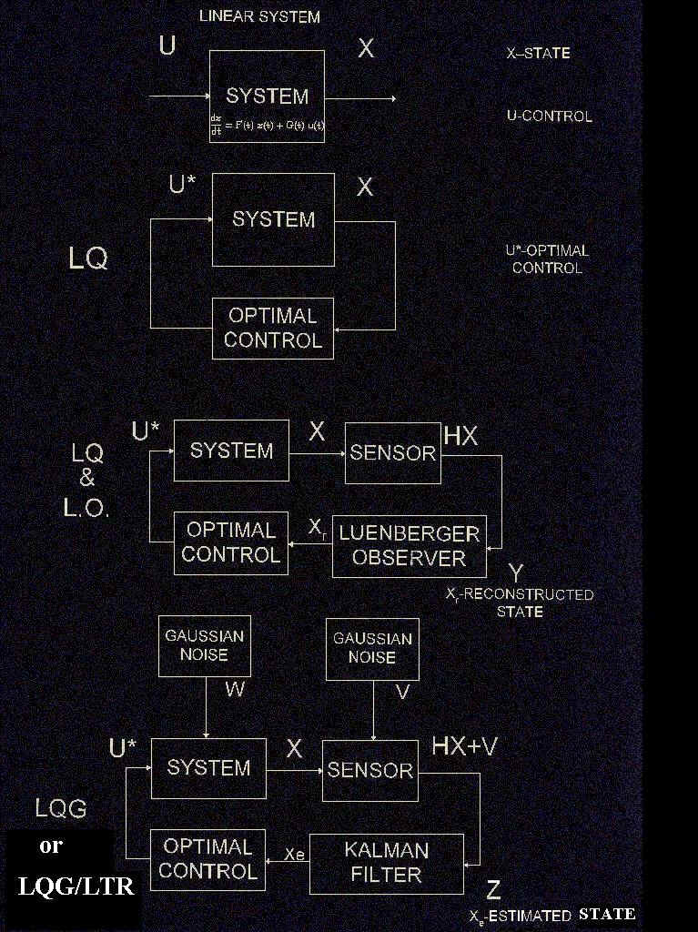


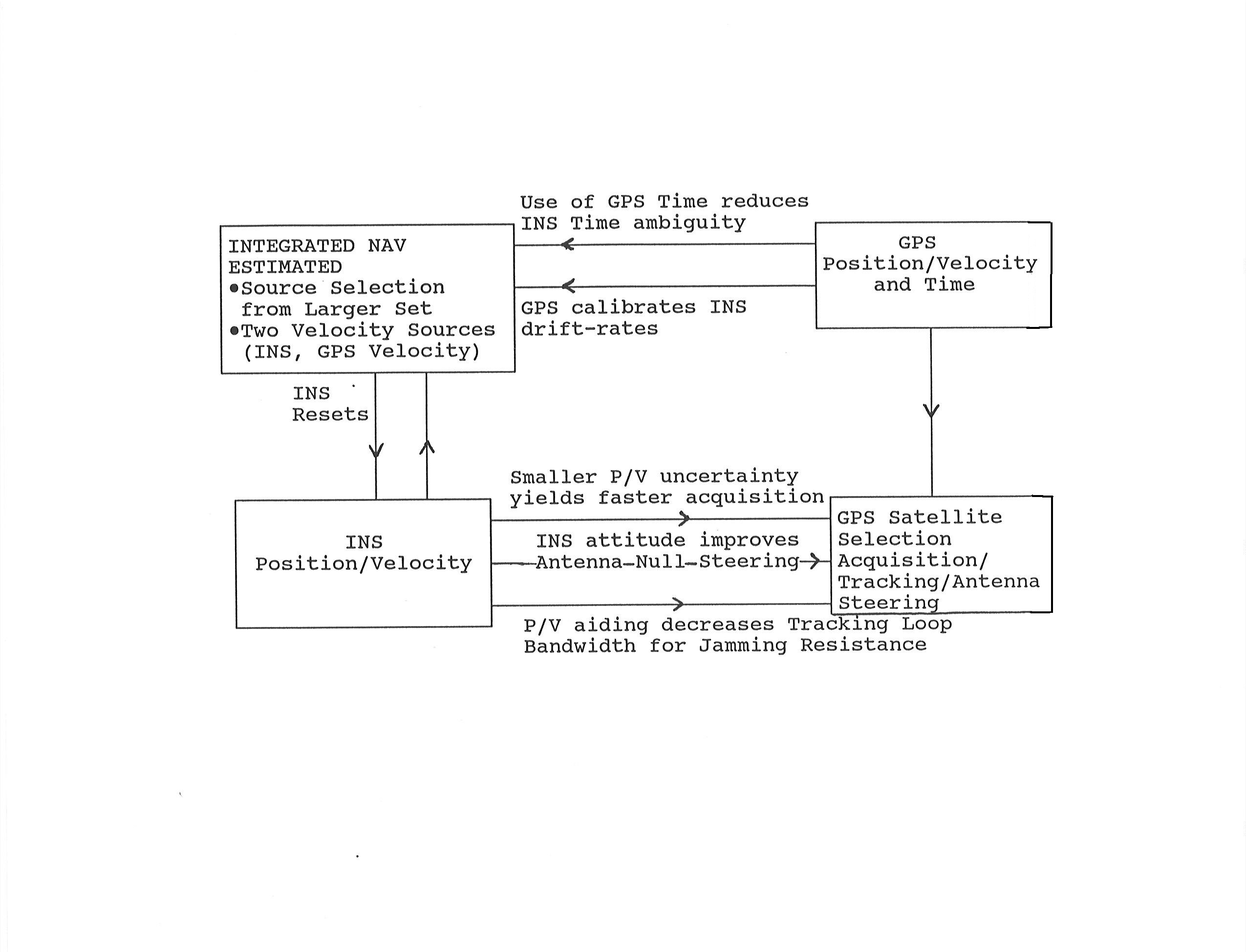

 Go
to Top
Go
to Top


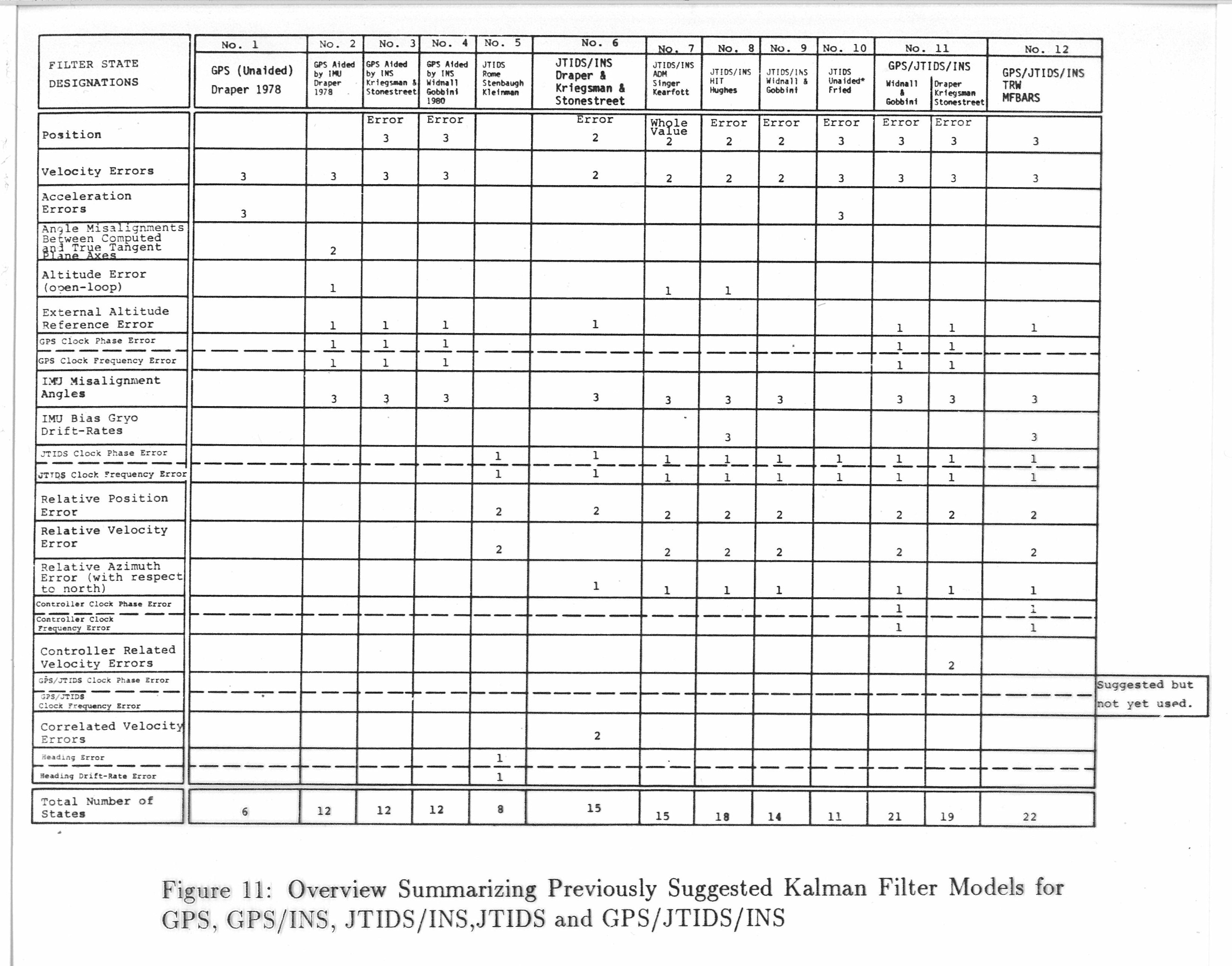


 but our frogs
eradicate them completely as they keep all programming bugs far
away from TK-MIP!
but our frogs
eradicate them completely as they keep all programming bugs far
away from TK-MIP!
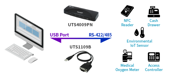